A conformal map locally preserves angles between directed curves as well as the orientation. In two dimensions, orientation-preserving conformal maps are locally invertible complex analytic functions, as we will discuss below. Our motivation here is to build the machinery to solve electrostatic and fluid flow problems. We will start from scratch and build towards fancy mappings to translate bizarre geometric boundaries to manageable ones.
Defining the complex derivative
Consider a function \(f\) defined on the complex plane as \(f(z)\) with \(z=x+iy\). The derivative of a function is defined by perturbing its argument by a small amount and computing the change in the function. In the case of complex variables, we can move \(z\) to \(z+\Delta z\), as illustrated in Fig. 1.
Figure 1: The position \(z\) in the complex plane is perturbed to a nearby point given by \(z+\Delta z\).
The complex derivative is defined just like in the case of familiar derivative: \[\begin{equation} \frac{df(z)}{dz}\equiv\lim_{\Delta z\rightarrow 0} \frac{f(z+\Delta z)-f(z)}{\Delta z}. \tag{1} \end{equation}\]
However, note that we are free to perturb the point as we wish. We can move it only vertically, that is \(\Delta z=i\Delta y\), or only horizontally , \(\Delta z=\Delta x\), or with any combination of these two. We require that the derivative is the same no matter how we move the point, and that is a strong requirement! In order to simplify the notation, let us split \(f(z)\) into its real and imaginary parts: \[\begin{equation} f(z)\equiv u(x,y)+iv(x,y) \tag{2}. \end{equation}\] Let us first calculate the derivative when we move the point horizontally: \(\Delta y=0\) and \(\Delta z=\Delta x\): \[\begin{equation} \frac{df(z)}{dz}=\lim_{\Delta x\rightarrow 0} \frac{f(z+\Delta x)-f(z)}{\Delta x} =\lim_{\Delta x\rightarrow 0} \frac{u(x+\Delta x,y)+iv(x+\Delta x,y) -u(x,y)-iv(x,y)}{\Delta x}=\frac{\partial u}{\partial x}+i\frac{\partial v}{\partial x}. \tag{3} \end{equation}\]
Secondly, we move the point vertically: \(\Delta x=0\) and \(\Delta z=i \Delta y\): \[\begin{equation} \frac{df(z)}{dz}=\lim_{ \Delta y\rightarrow 0} \frac{f(z+i \Delta y)-f(z)}{i \Delta y} =\lim_{\Delta y\rightarrow 0} \frac{u(x,y +\Delta y)+iv(x,y+\Delta y) -u(x,y)-iv(x,y)}{i \Delta y}=-i \frac{\partial u}{\partial y}+\frac{\partial v}{\partial y}. \tag{4} \end{equation}\] We want the results in Eqs. (3) and (4) to be the same which requires:
\[\begin{eqnarray} \frac{\partial u}{\partial x}&=&\frac{\partial v}{\partial y}\text{ and } \frac{\partial u}{\partial y}=-\frac{\partial v}{\partial x}. \tag{5} \end{eqnarray}\] Equations in (5) is known as Cauchy-Riemann equations, named after A. L. Cauchy who discovered them and G. F. B. Riemann who made them fundamental in the theory of functions of complex variables. Now take \(\partial_x\) of the first line and \(\partial_y\) of the second line to add them up together: \[\begin{eqnarray} \frac{\partial^2 u}{\partial x^2}+\frac{\partial^2 u}{\partial y^2}=0\tag{6} \end{eqnarray}\]
Similarly, take \(\partial_y\) of the first line and \(-\partial_x\) of the second line to add them up together: \[\begin{eqnarray} \frac{\partial^2 v}{\partial x^2}+\frac{\partial^2 v}{\partial y^2}=0\tag{7}. \end{eqnarray}\] In a shorter notation, we can write
\[\begin{eqnarray} \nabla^2 u=0 \text{ and } \nabla^2 v=0\tag{8}, \end{eqnarray}\] which is known as Laplace’s equation where \(\nabla^2=\partial^2_x+\partial^2_y.\)
Orthogonality
Let’s look at the equations in (5) from a different perspective.The gradients of \(u\) and \(v\) can be written in the vectorial for as \((u_x,u_y)\) and \((v_x,v_y)\), respectively. Now take the inner product of the gradients:
\[\begin{eqnarray} (u_x,u_y)^T\cdot (v_x,v_y) =u_x v_x+ u_y v_y=u_x(- u_y)+ u_y u_x= 0\tag{9}, \end{eqnarray}\] which shows that the gradients are orthogonal to each other. If their gradients are perpendicular so are their tangents, see the proof below.
Let’s prove that gradient vector is indeed perpendicular to the tangent. In a generic case, \(f\) can be a function of multiple variables: \(f=f(x_1,x_2,\cdots,x_n)\) where \(\mathbf{x}=(x_1,x_2,\cdots,x_n)\) is an \(n\) dimensional vector. The level surface of this function is composed of \(\mathbf{x}\) values such that \(f(\mathbf{x}_0)=k\), which defines an \(n-1\) dimensional level surface. What we want to prove is that for any point on the level surface, \(f(\mathbf{x}_0)=k\), the gradient of \(f\), i.e., \(\mathbf{\nabla}f\vert_{\mathbf{x}_0}\) is perpendicular to the surface.
Let us take an arbitrary curve on this surface, \(\mathbf{x}(t)\), parameterized by a parameter \(t\), and assume it passes through \(\mathbf{x}_0\) at \(t=t_0\). On the surface \(f(\mathbf{x}(t))=f\left(x_1(t),x_2(t),\cdots,x_n(t)\right)= k\). Let’s take the parametric derivative of \(f\) and apply the chain rule.
\[\begin{eqnarray} \frac{df}{dt}=0=\sum_{i=1}^n \left.\frac{\partial f}{\partial x_i}\right\vert_{\mathbf{x}_0}\left. \frac{d x_i}{dt}\right\vert_{t_0} = \left.\mathbf{\nabla} f\right\vert_{\mathbf{x}_0} \cdot \dot{\mathbf{x}}\vert_{t_0} \tag{10}, \end{eqnarray}\] where we defined \(\dot{\mathbf{x}}\vert_{t_0}=\left.\frac{d\mathbf{x}(t)}{dt}\right\vert_{t_0}\), which is nothing but the tangent line. Therefore we conclude that the gradient is perpendicular to the tangent lines on the surface.
This means that if we associate \(u(x,y)\) with an electric potential \(V(x,y)\), then the lines of constant \(v(x,y)\) are perpendicular to the \(u(x,y)\). This implies that \(v(x,y)\) equipotentials are the field lines of \(u(x,y)\). But note the symmetry between \(u\) and \(v\): how do we decide which one is the potential and which one is the field lines? We decide on that by looking at the symmetry of the problem and the boundary conditions. More on this later.
Conformal mapping
Consider two curves \(\xi\) and \(\gamma\). We will assume that they intersect at a point \(z_0\) as in Fig. 2.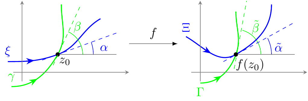
Figure 2: The position \(z\) in the complex plane is perturbed to a nearby point given by \(z+\Delta z\).
Let us first concentrate on the curve \(\xi\) and assume it is parameterized as \(z(t)\) with a parameter \(t\). This curve gets mapped by the function \(f\) onto the curve \(\Xi\):
\[\begin{equation} \tag{11} \Xi(t)=f(z(t)). \end{equation}\] We want to investigate the angle measured from the horizontal axis at the intersection point \(z_0=z(t_0)\). To this end, let’s compute the derivative with respect to the parameter \(t\): \[\begin{equation} \tag{12} \Xi'(t_0)=f'\left(z(t_0)\right)z'(t_0). \end{equation}\] We can look at the angle by taking the argument of Eq. (12): \[\begin{equation} \tag{13} \arg \Xi'(t_0)=\arg f'\left(z(t_0)\right)+ \arg z'(t_0). \end{equation}\] \(\arg f'\left(z(t_0)\right)\) is intrinsic to the mapping function \(f\). Let’s define this angle as \(\zeta\). \(\arg z'(t_0)\) is the angle of the tangent line, and in Fig. 2, we denoted that angle as \(\alpha\). We also denoted \(\arg \Xi'(t_0)\) as \(\tilde\alpha\). We can rewrite Eq. (13) in these angles as:
\[\begin{equation} \tag{14} \tilde\alpha=\zeta+ \alpha. \end{equation}\]
We can rinse and repeat the same exercise for the curve \(\gamma\) and its image \(\Gamma\) to get: \[\begin{equation} \tag{15} \tilde\beta=\zeta+ \beta. \end{equation}\] The profound observation here is that in Eqs. (14) and (15) we have the very same offset \(\zeta\), which corresponds to the angle associated with the the mapping \(f\) at \(z_0\). However, remember in the first section that the derivative in the complex plane is defined such that it is independent of how you approach \(z_0\). That is exactly why we get the same angle form the function \(f\) whether we evaluate it along the direction of \(\xi\) or \(\gamma\). If we take the difference of Eqs. (14) and (15) we get:
\[\begin{equation} \tag{16} \tilde\alpha-\tilde\beta=\alpha- \beta, \end{equation}\] which shows that the angle between the curves is preserved under such mappings.
A simple \(z\to z^2\) mapping is conformal and it is illustrated in Fig. 3.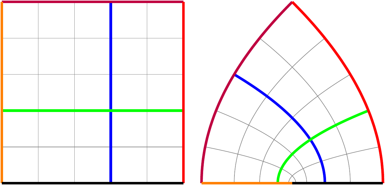
Figure 3: The mapping of the color coded Cartesian grid with function \(z^2\). Note how the grid lines curve and bend while preserving the angles at the intersection points.
Mapping harmonic functions
Consider a harmonic function \(\varphi(x,y)\) which satisfies \[\begin{eqnarray} \frac{\partial^2 \varphi}{\partial x^2}+\frac{\partial^2 \varphi}{\partial y^2}=0.\tag{17} \end{eqnarray}\] Assume we do a mapping from the complex variable \(z=x+i\,y\) with a function \(f\) such that \(f(z)=u(x,y)+i\, v(x,y)\). We want to describe how Eq. (17) will look like in the new coordinates \((u,v)\). We will assume that \(f(z)\) is analytic, i.e., it satisfies the Cauchy-Rieman conditions in Eq. (5), and furthermore we will assume \(|f'(z)|\neq 0\) in the domain of interest. Assuming a 1-1 mapping from \((x,y)\) to \((u,v)\), we can in principle find the inverse transformation, \(f^{-1}\) such that \(x\) and \(y\) can be expressed as functions of \(u\) and \(v\): \(x=x(u,v)\) and \(y=y(u,v)\). In other words \(\varphi\) can be expressed as a function of independent \(u\) and \(v\). It will look like this: \[\begin{eqnarray} \varphi(x,y)=\varphi\left(x(u,v),y(u,v)\right)\equiv\phi(u,v).\tag{18} \end{eqnarray}\] We want to understand what kind of equation \(\phi(u,v)\) could satisfy given all the assumptions above. Let’s shut up and calculate: \[\begin{eqnarray} \varphi_x&=& \phi_u u_x+\phi_v v_x,\\\nonumber \varphi_{xx}&=& \phi_u u_{xx}+\phi_v v_{xx}+(\phi_{uu}u_x+\phi_{uv}v_x )u_x+(\phi_{vu}u_x+\phi_{vv}v_x )v_x,\\\nonumber \varphi_y&=& \phi_u u_y+\phi_v v_y,\\\nonumber \varphi_{yy}&=& \phi_u u_{yy}+\phi_v v_{yy}+(\phi_{uu}u_y+\phi_{uv}v_y )u_y+(\phi_{vu}u_y+\phi_{vv}v_y )v_y, \tag{19} \end{eqnarray}\] from which we get: \[\begin{eqnarray} \varphi_{xx}+\varphi_{yy}&=& \phi_{uu}\left(u^2_x+u^2_y\right) +\phi_{vv}\left(v^2_x+v^2_y\right) +\phi_u \cancelto{0}{(u_{xx}+ u_{yy})} +\phi_v \cancelto{0}{(v_{xx}+ v_{yy})} +2 \phi_{uv}\cancelto{0}{(u_x v_x+u_y v_y)}\nonumber \\ &=&(\phi_{uu}+\phi_{vv})\left(u^2_x+v^2_x\right)=(\phi_{uu}+\phi_{vv})|f'(z)|^2=0\implies \phi_{uu}+\phi_{vv}=0. \tag{20} \end{eqnarray}\] This is very important: harmonic functions are mapped to harmonic functions when the mapping function is analytical with a non-vanishing derivative.
Complex potential
Let’s define the following analytical function: \[\begin{eqnarray} \Phi(z)=\phi +i\psi, \tag{21} \end{eqnarray}\] where \(\phi\) and \(\psi\) are assumed to be analytical. As we have seen in Sec. Orthogonality, gradients of \(\phi\) and \(\psi\) are perpendicular to each other: \[\begin{eqnarray} (\phi_x,\phi_y)^T\cdot (\psi_x,\psi_y) = 0\tag{22}, \end{eqnarray}\] which means the level lines are perpendicular too. We also define a vector quantity \(F\) as the gradient of \(\phi\): \[\begin{eqnarray} \mathbf F=\vec \nabla \phi= (\phi_x,\phi_y) \tag{23}. \end{eqnarray}\] The object \(\vec F\) is divergence and curl free: \[\begin{eqnarray} \vec \nabla \times \mathbf F= \phi_{yx}-\phi_{xy}=0,\nonumber\\ \vec \nabla \cdot \mathbf F= \phi_{xx}+\phi_{yy}=0. \tag{24} \end{eqnarray}\] This makes \(\vec F\) a compatible vector field for incompressible and irrotational flows and electrostatic problems.
Electrostatic problems
Let’s start with a very gentle problem. Consider an infinite line of charge along the vertical axis as illustrated in Fig. 4.
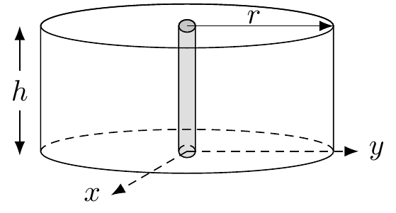
Figure 4: A segment of infinite line charge of density \(\lambda\) that lies along the \(z\)-axis. We put a hypotetical cylinder of height \(h\) and radius \(r\), co-centric with the line charge.
This is a text-book example for the application of the Gauss law to compute the electric field and the electrostatic potential. We will repeat this exercise at the context of complex functions. We start from the Gauss law: \[\begin{eqnarray} \mathbf{\nabla}\cdot\mathbf{E} &=& \frac{\rho}{\varepsilon_0} \tag{25}. \end{eqnarray}\] Integrating this equation over the volume of the cylinder, we get: \[\begin{eqnarray} \int_\mathcal{V}d^3x \mathbf{\nabla}\cdot\mathbf{E} &=& \int_\mathcal{\partial V}d\vec S \cdot\mathbf{E}= \int_\mathcal{\partial V}r d\phi d z \hat r \cdot \hat r E(r) = 2\pi r h E(r) \nonumber\\ &=&\frac{1}{\varepsilon_0} \int_\mathcal{V}d^3x \rho= \frac{Q_\text{enc}}{\varepsilon_0}=\frac{h \lambda}{\varepsilon_0} , \tag{26} \end{eqnarray}\] from which we get: \[\begin{eqnarray} E(r) = \frac{ \lambda}{2\pi \varepsilon_0 \, r} . \tag{27} \end{eqnarray}\] The corresponding electrostatic potential reads: \[\begin{eqnarray} V(r)= -\int_{r_0}^r d\vec{r}'\cdot \vec{E}(r') = -\frac{ \lambda}{2\pi \varepsilon_0 \, }\ln\left(\frac{r}{r_0}\right). \tag{28} \end{eqnarray}\] We can actually drop \(\ln(r_0)\) term as it is a constant and simplify the potential to: \[\begin{eqnarray} V(r)= -\frac{ \lambda}{2\pi \varepsilon_0 }\ln\left(r\right). \tag{29} \end{eqnarray}\] The corresponding electric field is the negative gradient of \(V(r)\): \[\begin{eqnarray} \vec E(r)= -\vec \nabla V(r)= \frac{ \lambda}{2\pi \varepsilon_0 r}\hat r. \tag{30} \end{eqnarray}\]
We can equivalently solve this directly from the Poisson equation in the cylindrical coordinates, and we looked into that problem in an earlier post.
The two-dimensional view of the potential and the electric-field is shown in Fig. 5.
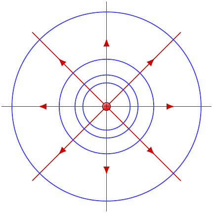
Figure 5: The radial electric fields and the co-centric equipotential lines.
The electric fields are in radial direction, and they are perpendicular to the equipotential lines. We want to resolve the problem in the context of complex variables using a conformal map. We want to find the function \(\varphi(x,y)\) which satisfies Eq. (17). This requires solving the Laplace equation in cylindrical coordinates as we just did. However, even without solving the problem, due to the symmetry, we know the electric potential lines have to be circles and the electric fields have to be the radial lines. We want to map the circles and rays into a simpler view in the mapped space. The circles in the complex plane are represented by \(z=r e^{i\theta}\). As it has a built-in exponential, intuitively we can see that we can undo that if we tried \(f(z)=\ln(z)\) as the mapping function. \[\begin{eqnarray} f(z) = \ln(z)= \ln(r)+ i \theta\equiv u +i v. \tag{31} \end{eqnarray}\] This maps \((x,y)\) to \((u,v)\). Furthermore the harmonic feature of \(\varphi\) with respect to \((x,y)\) is still valid for \(\phi\) with respect to \((u,v)\).
Figure 6 shows that circles on the right are mapped to vertical lines in the \((u,v)\) space.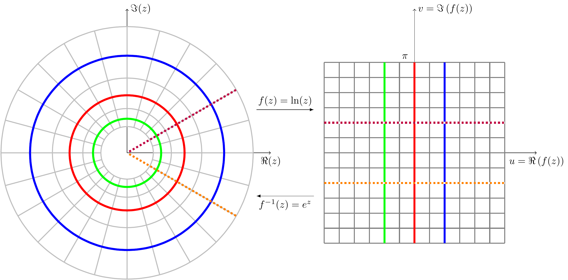
Figure 6: The mapping with the function \(\ln (z)\) and its invers \(e^z\).
The Laplace equation in the \((u,v)\) space couldn’t be any easier:
\[\begin{eqnarray} (\partial^2_u +\partial^2_v)\phi=0 \tag{32}. \end{eqnarray}\] We can impose the boundary conditions at the red (\(u=0\)) curve and at the blue curves \(u\equiv 1\) with \(\phi(0)\equiv0\) and \(\phi(u=1)=\phi_1\). With these boundary conditions we get: \[\begin{eqnarray} \phi(u)= \phi_1 u\tag{33}. \end{eqnarray}\] Finally, we revert \(u\) to \((r,\theta)\) coordinates using Eq. (31): \(u=\ln(r)\), which implies \[\begin{eqnarray} \varphi(r)= \phi_1 \ln(r)\tag{34}. \end{eqnarray}\]