TL;DR
This post is a quantitative analysis of the concepts discussed in Veritasium’s The Big Misconception About Electricity video, and it is going to be a long one. Here is the summary of the post for “Too long; didn’t read!” folks:
- All the energy transfer between circuit elements is done only by electric fields.
- Magnetic fields do not transfer energy to charged particles, you can completely ignore them.
- The Poynting vector is relevant only when you are specifically interested in the energy and momentum of the electromagnetic fields.
- The circuit in the video and its generalized versions can be solved analytically, see the section Solving Veritasium’s circuit analytically.
- If you want to skip the math and just play with the interactive plots, see the section Build your own circuit.
- Bonus: Changing magnetic fields do not induce electric fields!
- Update: Veritasium has released a new video, see the section The follow up video.
In a direct current(DC) circuit the Poynting vector is a red herring. Sure, it is mathematically consistent but physically it is completely redundant. Trying to explain energy flow in a circuit, particularly when it is DC, using the Poynting vector is not a very good choice since it obscures the real underlying process. Energy transport from a battery to a load can be explained in a much clearer way without ever invoking the Poynting vector or magnetic fields. This is exactly what I will discuss in this post with rigorous math and physics. I will also dedicate a good chunk of the post to a generalized version of the circuit in the video in the context of transmission lines.
Buckle up and enjoy!
Introduction
I would like to say a few words on the video from Veritasium titled The Big Misconception About Electricity, and other similar videos1 which motivate the use of the Poynting vector to explain energy transfer in an electrical circuit. I suggest you watch the video first and come back to read the post.
The Big Misconception About Electricity, Veritasium
Below is my summary of the video:
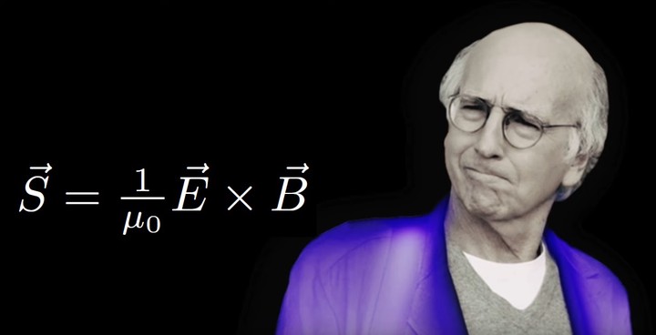
It starts with a seemingly tricky question on a simple circuit, and then delves into photons with the oscillating electric (\(\mathbf {E}\) ) and magnetic (\(\mathbf B\) ) fields to motivate the Poynting vector, \(\mathbf S=\frac{1}{\mu_0}\mathbf {E}\times \mathbf B\), which happens to be in the direction of the photon propagation. Then says: “… But the kicker is this, Poynting equation doesn’t just work for light, it works anytime there are electric and magnetic fields coinciding. …” to circle back to the circuit to argue the following: The flow of energy is given by the Poynting vector. If you calculate that vector by crossing \(\mathbf {E}\) and \(\mathbf B\) fields on the battery side, it points away from the battery. If you calculate it on the load side, it points into the load. Therefore the battery pumps energy to the field, and that energy is carried to the load along the lines of the \(\mathbf S\) vector and gets delivered to the load.
I believe some parts of the video are misleading and they create more misconceptions. Here I will try to present the full math and physics behind the Poynting theorem and the telegraph line. So let this be the warning that there will be some calculus involved! Let’s first discuss how energy is moved between the fields and the electrons.
Which field transfers energy?
If you apply a force \(\mathbf {F}\) on a particle, and move it by a small distance \(d \mathbf {x}\,\), the increase in the mechanical energy is \(du_\text{mec}=\mathbf {F}\cdot d \mathbf {x}\,\). This can be re-written as \(du_\text{mec}=\mathbf {F}\cdot \frac{d \mathbf {x}\,}{dt} dt=\mathbf {F}\cdot\mathbf {v} dt\), where \(\mathbf {v}\) is the velocity vector and \(dt\) is the differential time. The force on a particle of charge \(q\) moving in \(\mathbf {E}\) and \(\mathbf B\) fields is known as the Lorentz force and it is given by: \[\begin{eqnarray} \mathbf{F}= q(\mathbf{E} + \mathbf{v} \times \mathbf{B}). \tag{1} \end{eqnarray}\]
Magnetic fields are lazy
One thing you notice in Eq. (1) is that the force associated with the magnetic field is perpendicular to the velocity vector \(\mathbf {v}\), which becomes very important when we compute the work done on the charge: \[\begin{eqnarray} \frac{du_\text{mec}}{dt}= \mathbf {F}\cdot \mathbf {v} = q\left(\mathbf {E} \cdot \mathbf {v} + (\mathbf {v} \times \mathbf B) \cdot \mathbf {v} \right)=q \mathbf {E} \cdot \mathbf {v}. \tag{2} \end{eqnarray}\] Note how the magnetic field vector disappeared from the energy equation. This is not surprising at all since it is a well-known fact that magnetic fields do not do work on moving charges. They just sit there and do nothing to transfer energy. They are irrelevant for calculations of energy transfer between field and charges. This is similar to swinging a stone tied to a rope at a constant angular speed in a circular motion. The force on the string is radial whereas the movement is in the angular direction. You are not making it go any faster; you are not giving it any extra energy. The tension on the string just changes the direction of the velocity, not its magnitude.
Electric fields do all the work
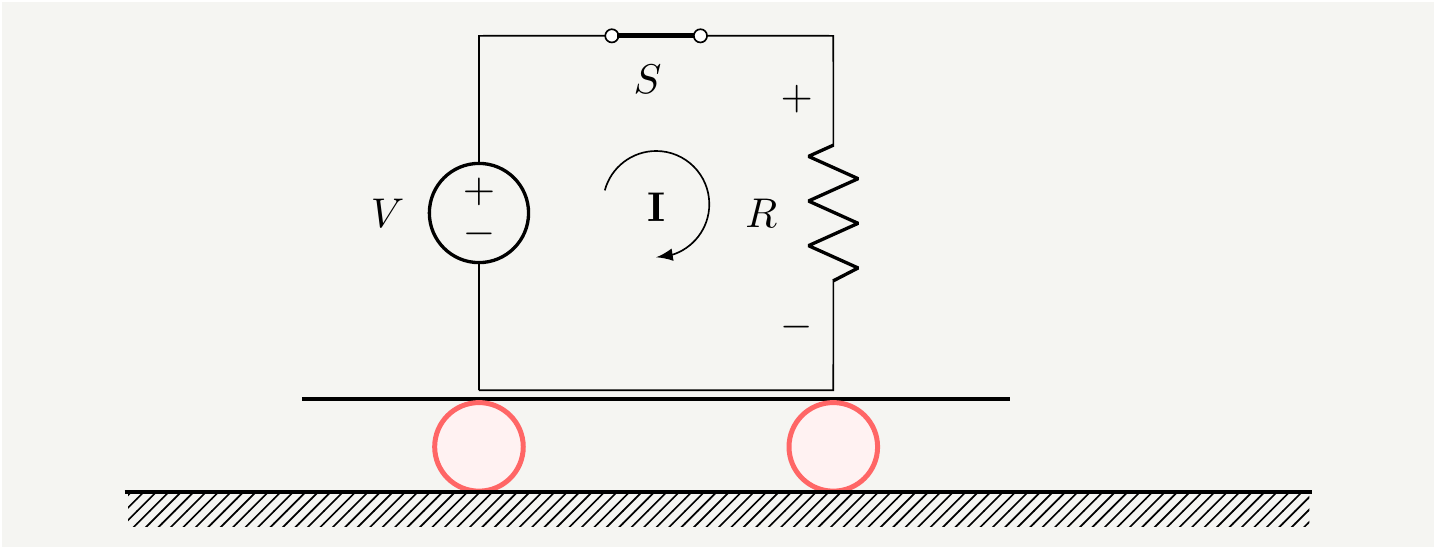
We can write \(q\), the amount of charge moved by the electric field, as \(\rho d^3\mathbf {x}\,\) where \(\rho\) is the charge density. Therefore, the total change of energy in an arbitrary domain \(\Omega\) can be written as \[\begin{eqnarray} \frac{dU_\text{mec}}{dt}\equiv \int_\Omega d^3 \mathbf {x}\, \frac{du_\text{mec}}{dt}= \int_\Omega d^3\mathbf {x}\,\, \mathbf {E} \cdot \mathbf {J}, \tag{3} \end{eqnarray}\] where we defined the charge density vector \(\mathbf {J}\) as : \[\begin{eqnarray} \mathbf {J} \equiv\rho \mathbf {v}. \tag{4} \end{eqnarray}\] Equation (3) is very neat and simple, yet so powerful: it tells you everything you need to know about the transfer of energy from fields to matter and back. It is also localized to where currents exist. All the transfer of power in a circuit happens on the elements that carry current and electric field simultaneously. Electric field delivers energy to charges if the current density \(\mathbf {J}\) is aligned with the \(\mathbf {E}\) field. It extract energy from them if they are anti-parallel. Consider the following simple circuit:
Figure 1: A resistor connected as a load to a battery through a switch.
On the battery side, \(\mathbf {J}\) and \(\mathbf {E}\) vectors are anti-parallel, which means \(\frac{dU_\text{mec}}{dt}\) in Eq. (3) is negative. This makes perfect sense. The internal energy of the battery is decreasing, because it is transferred to the electron energy in the electric field. If it helps, you can visualize it as electrons climbing up in a potential, which requires energy. That is the energy provided by the battery. All the electrons connected to the negative terminal of a battery with a wire of negligible resistance have the very same potential. They have acquired the same energy to be at that potential. If you look at the same equation on the load side, the right hand side becomes positive. That means the energy of the material is increasing, which is another way of saying electrons are picking up energy. If it is a resistor, the energy ends up being converted to heat due to collisions.
Is there any work done inside the conducting wires? No, because the electric field inside the wires is very small. If we ignore resistance, there is no electric field in the wires at all, and the electrons are slowly drifting in the wire, as pointed out in the video by Dr. Bruce Hunt:… For most people and I think to this day, it’s quite counter-intuitive to think that the energy is flowing through the space around the conductor but the energy is, which is traveling through the field is going quite fast. How far do the electrons go? In this little thing you are talking about, they barely move. They don’t probably move at all.
I would like to pick up on a specific part of the his comment “… they[electrons] barely move.” This feeds into the overall narrative of the video which suggests that it is not about what happens inside the wires, it is all about the fields, and electrons are almost irrelevant. Look how slow they move- they have almost no energy.
This couldn’t be further from the truth:
- First of all, all the fields are created by the electrons, therefore, it is, by definition, all about what happens to the electrons.
- Furthermore, if you are interested in the transfer of energy from the source to the load, every relevant thing happens inside the wires and circuit elements.
- Although electrons are moving slowly in the conducting wires, that is not the case everywhere in the circuit. There are places they move very very fast.
While the electrons drift very slowly in the conducting wires, they accelerate once they arrive at the load, because there is a large potential difference, hence a large electric field. Consider a voltage of difference of \(100V\). Electrons have a mass of \(9\times 10^{-31}\) kg and a charge of \(1.6\times 10^{-19}\) C. An electron that accelerates under \(100V\) could reach to a speed of \(v=\sqrt{\frac{2 q V}{m}}=6\times10^6 m/s\). That is some speed! Obviously, their speed speed won’t reach to these values since electrons will hit on some obstacles in the resistor, and they will slow down by converting the kinetic energy to heat. And that is exactly how the energy is delivered to the load. If the load is a light emitting diode(LED), the electron will shoot out a photon to release the energy. That electron then drops to the positive terminal of the load, into the conductor and it will start drifting slowly back to the source.
I will leave the discussion here for now, but we will come back to this later. Let’s first derive the Poynting theorem.
The Poynting Theorem
There are cases Poynting theorem comes handy. For example, consider a case where you sit away from the static charges (\(\rho\)), and currents (\(\mathbf {J}\)), and you don’t exactly know how they behave. However, you have a device that can measure \(\mathbf {E}\) and \(\mathbf B\). Since \(\mathbf {E}\) and \(\mathbf B\) are created by the charges and we should be able the revert the relation to write \(\rho\) and \(\mathbf {J}\) in terms of the fields they create. This is done by using Maxwell’s equations, which are shown below: \[\begin{eqnarray} \text{Gauss' Law for electric fields:}\qquad \mathbf{\nabla}\cdot\mathbf{E} &=& \frac{\rho}{\varepsilon_0}, \tag{5} \end{eqnarray}\] \[\begin{eqnarray} \text{Gauss' Law for magnetic fields:}\qquad \mathbf{\nabla}\cdot\mathbf{B} &=& 0 \tag{6}, \end{eqnarray}\] \[\begin{eqnarray} \text{Faraday's Law:}\qquad \mathbf{\nabla}\times\mathbf{E} &=& -\frac{\partial \mathbf{B}}{\partial t} \tag{7}, \end{eqnarray}\] \[\begin{eqnarray} \text{Ampere's Law:}\qquad \mathbf{\nabla}\times\mathbf{B} &=& \mu_0\mathbf{J}+\mu_0\varepsilon_0\frac{\partial\mathbf{E}}{\partial t} \tag{8}. \end{eqnarray}\] We can isolate \(\mathbf {J}\) from Eq. (8) as: \[\begin{eqnarray} \mathbf{J} &=& \frac{1}{\mu_0}\mathbf{\nabla}\times\mathbf{B} -\varepsilon_0\frac{\partial\mathbf{E}}{\partial t}. \tag{9} \end{eqnarray}\] Pause for a moment to contemplate what this means: we are trading the localized source current \(\mathbf {J}\) with a certain function of the fields it creates, which are not localized. \(\mathbf {E}\) and \(\mathbf B\) fields extend beyond the localized charges, technically they extend out to infinity. Let’s take \(\mathbf {J}\) from Eq. (9) and stick it back into Eq. (3) to get: \[\begin{eqnarray} \frac{dU_\text{mec}}{dt}= \int_\Omega d^3\mathbf {x}\,\, \mathbf {E} \cdot \left(\frac{1}{\mu_0}\mathbf{\nabla}\times\mathbf{B} -\varepsilon_0\frac{\partial\mathbf{E}}{\partial t}\right). \tag{10} \end{eqnarray}\] We have to do some vector calculus for the first term in the integrand: \[\begin{eqnarray} \mathbf {E} \cdot \left(\mathbf{\nabla}\times\mathbf{B} \right)&=& \mathbf {E}^i\epsilon^{ijk}\mathbf{\nabla}^j\mathbf{B}^k=\mathbf{\nabla}^j\left(\mathbf {E}^i\epsilon^{ijk}\mathbf{B}^k\right)-\mathbf{\nabla}^j\mathbf {E}^i\epsilon^{ijk}\mathbf{B}^k=\mathbf{B}\cdot \left( \mathbf{\nabla} \times \mathbf{E} \right)-\mathbf{\nabla}\cdot \left( \mathbf{E} \times \mathbf{B} \right)\nonumber\\ &=&-\mathbf{B}\cdot \frac{\partial \mathbf{B}}{\partial t} -\mathbf{\nabla}\cdot \left( \mathbf{E} \times \mathbf{B} \right), \tag{11} \end{eqnarray}\] where \(\epsilon^{ijk}\) is the Levi-Civita symbol, and summations over the repeated indices are implied. Also noting the equality \(\mathbf{V}\cdot \frac{\partial \mathbf{V}}{\partial t}=\frac{1}{2}\frac{\partial\mathbf{V}^2}{\partial t}\) for any vector \(\mathbf{V}\), we can re-write Eq. (10) as: \[\begin{eqnarray} \frac{dU_\text{mec}}{dt}= -\int_\Omega d^3\mathbf {x}\,\, \left( \frac{\partial}{\partial t}\left[ \frac{\varepsilon_0}{2}\mathbf {E}^2 + \frac{1}{2 \mu_0} \mathbf {B}^2\right] +\frac{1}{\mu_0} \mathbf{\nabla}\cdot \left[ \mathbf{E} \times \mathbf{B} \right]\right). \tag{12} \end{eqnarray}\] Finally we can use the divergence theorem to convert the volume integral of the divergence to the closed surface integral to get: \[\begin{eqnarray} \frac{dU_\text{mec}}{dt}= -\frac{\partial}{\partial t}\int_\Omega d^3\mathbf {x}\,\, \left( \frac{\varepsilon_0}{2}\mathbf {E}^2 + \frac{1}{2 \mu_0} \mathbf {B}^2 \right) -\frac{1}{\mu_0} \oint_{\partial\Omega} \left( \mathbf{E} \times \mathbf{B} \right)\cdot d \mathbf{A}. \tag{13} \end{eqnarray}\] We identify the following terms as the energy density of EM fields: \[\begin{eqnarray} \frac{\varepsilon_0}{2}\mathbf {E}^2 + \frac{1}{2 \mu_0} \mathbf {B}^2 \equiv u_\text{EM} \tag{14}, \end{eqnarray}\] and define \[\begin{eqnarray} \mathbf{S}\equiv\frac{1}{\mu_0} \mathbf{E} \times \mathbf{B}. \tag{15} \end{eqnarray}\] We can now finalize the energy continuity equation: \[\begin{eqnarray} \frac{d}{dt}(U_\text{mec}+U_\text{EM})= - \oint_{\partial\Omega} \mathbf{S}\cdot d \mathbf{A}, \tag{16} \end{eqnarray}\] where \(U_\text{EM}\equiv\int_\Omega d^3\mathbf {x}\, u_\text{EM}\). If you prefer the differential forms and densities, it will be as follows: \[\begin{eqnarray} \frac{d}{dt}(u_\text{mec}+u_\text{EM})= - \mathbf{\nabla}\cdot \mathbf{S}. \tag{17} \end{eqnarray}\] Equations (16) and (17) tell us that the change in the total energy, mechanical + electromagnetic, at a given point in space is given by the flux of electromagnetic energy, namely the Poynting vector. This is a great result, and it is typically used in circuits with high frequency currents due to the oscillating fields. Antennas are very good examples. You can compute the flux of out going fields in a transmitter, or the flux of incoming fields in a receiver. It is very convenient is such cases.
Poynting vector is not unique
As we went through the math and the change of variables, something might have leaked through the cracks. One thing we did without proper justification was to define the energy of the EM field as in Eq. (14). The motivation for it was that it matches the static case. However, it could be different for time dependent cases. This point is raised by Feynman in his lecture notes:…Before we take up some applications of the Poynting formulas [Eqs. (14) and (15)], we would like to say that we have not really “proved” them. All we did was to find a possible “\(u_\text{EM}\)” and a possible “\(\mathbf{S}\).” How do we know that by juggling the terms around some more we couldn’t find another formula for “\(u_\text{EM}\)” and another formula for “\(\mathbf{S}\)?” The new \(\mathbf{S}\) and the new u would be different, but they would still satisfy Eq. (17). It’s possible. It can be done, but the forms that have been found always involve various derivatives of the field (and always with second-order terms like a second derivative or the square of a first derivative). There are, in fact, an infinite number of different possibilities for \(u_\text{EM}\) and \(\mathbf{S}\) , and so far no one has thought of an experimental way to tell which one is right! People have guessed that the simplest one is probably the correct one, but we must say that we do not know for certain what is the actual location in space of the electromagnetic field energy. So we too will take the easy way out and say that the field energy is given by Eq. (14). Then the flow vector \(\mathbf{S}\) must be given by Eq. (15).
Feynman goes into the fact that there has been no experimental evidence to determine the exact form of the EM energy, but it is acceptable to use the simplest form, which also agrees with the static case. The point here is that there is some ambiguity in the definition of the \(u_\text{EM}\) and that ties into the ambiguity in \(\mathbf{S}\). I think it is a reasonable thing to assume Eq. (14) is valid.
Also note that \(\mathbf{S}\) is always accompanied by the divergence operator \(\mathbf{\nabla}\), or a closed surface integral. This means that, although the graphics showing \(\mathbf{S}\) field looks interesting, what counts is the divergence of it, and not surprisingly, for static circuits, the divergence is zero everywhere except for the battery and the load.
More importantly, the continuity relation in Eq. (17) constrains \(\mathbf{\nabla}\cdot \mathbf{S}\), the divergence of the Poynting vector, not \(\mathbf{S}\) itself directly. However, from fundamental theorem of vector calculus, also known as Helmholtz decomposition[1], we know that any vector field can be decomposed as the sum of the curl free part and the divergence free part. In other words, we can add \(\mathbf{\nabla}\times \mathbf{V}\), where \(\mathbf{V}\) is an arbitrary vector field, to \(\mathbf{S}\), and since \(\mathbf{\nabla}\cdot(\mathbf{\nabla}\times \mathbf{V})=0\), the continuity equations would be unaffected. This tells us that \(\mathbf{S}\) has a large redundancy built in. Due to the ambiguities above, people have come up with many different alternatives to the Poynting vector, see Ref.[2] for a historical compilation. Let me be clear, I am not disputing the validity of the Poynting vector, I am just pointing out the fact that it can be put in very different forms with different interpretations without changing the end physics.
\(\mathbf S\) is totally redundant for photons
One may think that a legitimate case to use the vector \(\mathbf S\) is the case of photons, as it kindly tells you the direction of the energy flux. I beg to differ. No one needs a new vector, \(\mathbf S\), to describe the direction of the energy carried by a photon. It is manifestly obvious that photons carry their energy in the direction they go. Let’s call the momentum vector of the photon as \(\mathbf{k}\) and consider the following illustration(reproduced from [3]):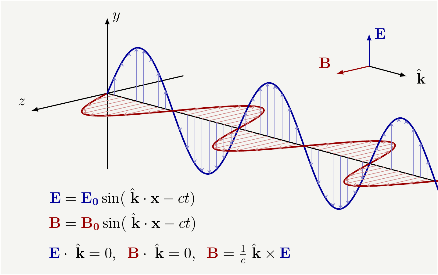
Figure 2: A cartoon for a planar EM field. The momentum vector, \(\mathbf{k}\), can be used as the energy flux for the photon.
The electric field and the magnetic field of a photon are perpendicular to each other and they are also perpendicular to the direction of the motion. These two requirements already consume all three orthogonal directions: any other vector you define can be decomposed in the basis of \(\mathbf {E}\), \(\mathbf B\), and \(\mathbf k\). So there is absolutely no need to invent a new vector to tell you the direction of the energy flow as you already know it is in the direction of \(\mathbf k\). Therefore \(\mathbf S\) is \(100\%\) redundant for the case of photons; you may use it if you’d like, but you most certainly don’t need it.
From \(\mathbf S\) back to matter
How is the electromagnetic energy described by \(\mathbf S\) gets converted back to the energy form we observe at the load? Let say it is a resistor; how does it heat up? What is the physical mechanism that extracts the energy from \(\mathbf S\)? That is actually a very important question, and it will shed some light into the redundancy of the \(\mathbf S\) for energy transfer calculations in a circuit. If you just take a closer look at the math, you can clearly see that \(\mathbf S\) dissolves into the good-old electric field coupled to the moving charges. This is kind of hilarious because we have to undo everything we did to get to the Poynting theorem. From Eq. (16), we know that the rate of energy delivered by the \(\mathbf S\) to a domain \(\Omega\) is: \[\begin{eqnarray} - \oint_{\partial\Omega} \mathbf{S}\cdot d \mathbf{A}&=&-\frac{1}{\mu_0} \int_\Omega d^3\mathbf {x}\,\, \mathbf{\nabla}\cdot \left( \mathbf{E} \times \mathbf{B} \right) =\frac{1}{\mu_0} \int_\Omega d^3\mathbf {x}\,\left(\mathbf {E} \cdot \left(\mathbf{\nabla}\times\mathbf{B} \right) +\mathbf{B}\cdot \frac{\partial \mathbf{B}}{\partial t} \right)\nonumber\\ &=&\frac{1}{\mu_0} \int_\Omega d^3\mathbf {x}\,\left[\mathbf {E} \cdot \left(\mu_0\mathbf{J}+\mu_0\varepsilon_0\frac{\partial\mathbf{E}}{\partial t} \right) +\mathbf{B}\cdot \frac{\partial \mathbf{B}}{\partial t} \right] =\frac{\partial}{\partial t}\int_\Omega d^3\mathbf {x}\,\, \left( \frac{\varepsilon_0}{2}\mathbf {E}^2 + \frac{1}{2 \mu_0} \mathbf {B}^2 \right)+ \int_\Omega d^3\mathbf {x}\,\mathbf {E} \cdot \mathbf{J}\nonumber\\ &=&\frac{d u_\text{EM}}{dt}+\frac{d u_\text{mec}}{dt}. \tag{18} \end{eqnarray}\] This shows again that \(\mathbf{S}\) feeds the energy to the magnetic and electric fields. It also feeds the energy to the matter. However, note how clearly separated these two things are: so if you are after the energy delivered to your resistor, just use \(\mathbf {E} \cdot \mathbf{J}\), there is absolutely no reason to bundle \(\mathbf{B}\) into your equations only to unpack them at the end to find out that it was totally irrelevant.
A couple of other observations:
- For a static circuit \(u_\text{EM}\) is constant. There are fields inside and around the circuit, and they don’t change at all. If we pursue the energy equations with the Poynting vector, we are shuffling around constant terms related to the fields, and they are always under a time derivative, which obviously gives zero.
- Even in the case of time dependent current, complicated part of the \(\mathbf{S}\) feeds into maintaining the fields outside the wires. If you are only interested in the power delivered to your load, you can just ignore the noise and compute \(\mathbf {E} \cdot \mathbf{J}\) at the load. If you want to compute power somewhere outside the wires, which is routinely done in AC circuit design, you are by default computing the power associated with the fields. Even in those cases you will most probably find that \(\mathbf{S}\) can be expressed in terms of more fundamental quantities.
Curl your Poynting vector
As we argued above, \(\mathbf{S}\) as defined in (15), is redundant when it is used to explain energy transport from a source to a load since it mixes in the energy associated with the fields. We have shown in Eq. (18) that the energy carried into a volume by \(\mathbf{S}\) can be decomposed explicitly into the EM piece and the energy delivered to the load. Can we split \(\mathbf{S}\) itself into two pieces in a vectorial form and identify the pieces go into the field and the load?
In the static case, electric field can be written as the gradient of a potential: \(\mathbf{E}=-\mathbf{\nabla}\phi\). Using this in the definition of the \(\mathbf{S}\) we get[4], [5]: \[\begin{eqnarray} \mathbf{S}&=& \frac{1}{\mu_0} \mathbf{E} \times \mathbf{B}=- \frac{1}{\mu_0}\mathbf{\nabla}\phi \times \mathbf{B}=-\frac{1}{\mu_0}\mathbf{\nabla}\times(\phi\mathbf{B} )+\frac{1}{\mu_0}\phi\mathbf{\nabla}\times\mathbf{B}=-\frac{1}{\mu_0}\mathbf{\nabla}\times(\phi\mathbf{B} )+\phi\mathbf{J}, \tag{19} \end{eqnarray}\] where we used Eq. (8). There is so much to like about this equation:
The first vector, \(\mathbf{\nabla}\times(\phi\mathbf{B} )\) is associated with the energy flux of the field, and it comes as a curl! Why is that important? It is critical because it is guaranteed to be divergence free: \(\mathbf{\nabla}\cdot \left(\mathbf{\nabla}\times(\phi\mathbf{B} )\right)=0\). This means that it delivers no energy to any volume: \[\begin{eqnarray} \oint_{\partial\Omega} \left(\mathbf{\nabla}\times(\phi\mathbf{B} )\right)\cdot d \mathbf{A}=\int_\Omega d^3\mathbf {x} \mathbf{\nabla}\cdot \left(\mathbf{\nabla}\times(\phi\mathbf{B} )\right)=0. \tag{20} \end{eqnarray}\] We can legitimately curl a part of the Poynting vector away, which also explains the title of this post!
We can identify \(\phi\mathbf{J}\) as the flux of energy to be delivered to the load. You may think this is problematic because \(\mathbf{J}\) is the current density and it circles back to the source. However once you notice that \(\mathbf{J}\) is accompanied by \(\phi\), which is the electrical potential, it makes perfect sense. The electric potential in Fig. 1 is \(V\) at the top, and \(0\) at the bottom wire. This vector is a one way, localized flux! It will actually make even more sense if we unpack \(\phi\mathbf{J}\) as \(\phi\rho \mathbf {v}\) as in Eq. (4): this is simply a flux of charges with potential energy \(\phi \rho\) at velocity \(\mathbf {v}\). We can also show that it is the part that delivers the power to the load:
\[\begin{eqnarray} \oint_{\partial\Omega} \phi\mathbf{J} \cdot d \mathbf{A}=\int_\Omega d^3\mathbf {x} \mathbf{\nabla}\cdot \left(\phi\mathbf{J}\right)= \int_\Omega d^3\mathbf {x} \left(\mathbf{\nabla}\phi\cdot \mathbf{J} +\phi\cancelto{0}{\mathbf{\nabla}\cdot\mathbf{J}}\right) =-\int_\Omega d^3\mathbf {x} \mathbf{E}\cdot \mathbf{J}, \tag{21} \end{eqnarray}\] which is precisely the starting point of the derivation for the Poynting theorem, see Eq. (3). It turns out, after all, that it is still legitimate to say that the power the load receives comes within the wire.
Free energy and a bootstrap rocket?
One strange consequence of Poynting theorem is that it implies a non-vanishing energy-momentum flux even for static electric and magnetic fields. Let’s investigate this weirdness a bit. Consider following simple set up with an electromagnet and a capacitor: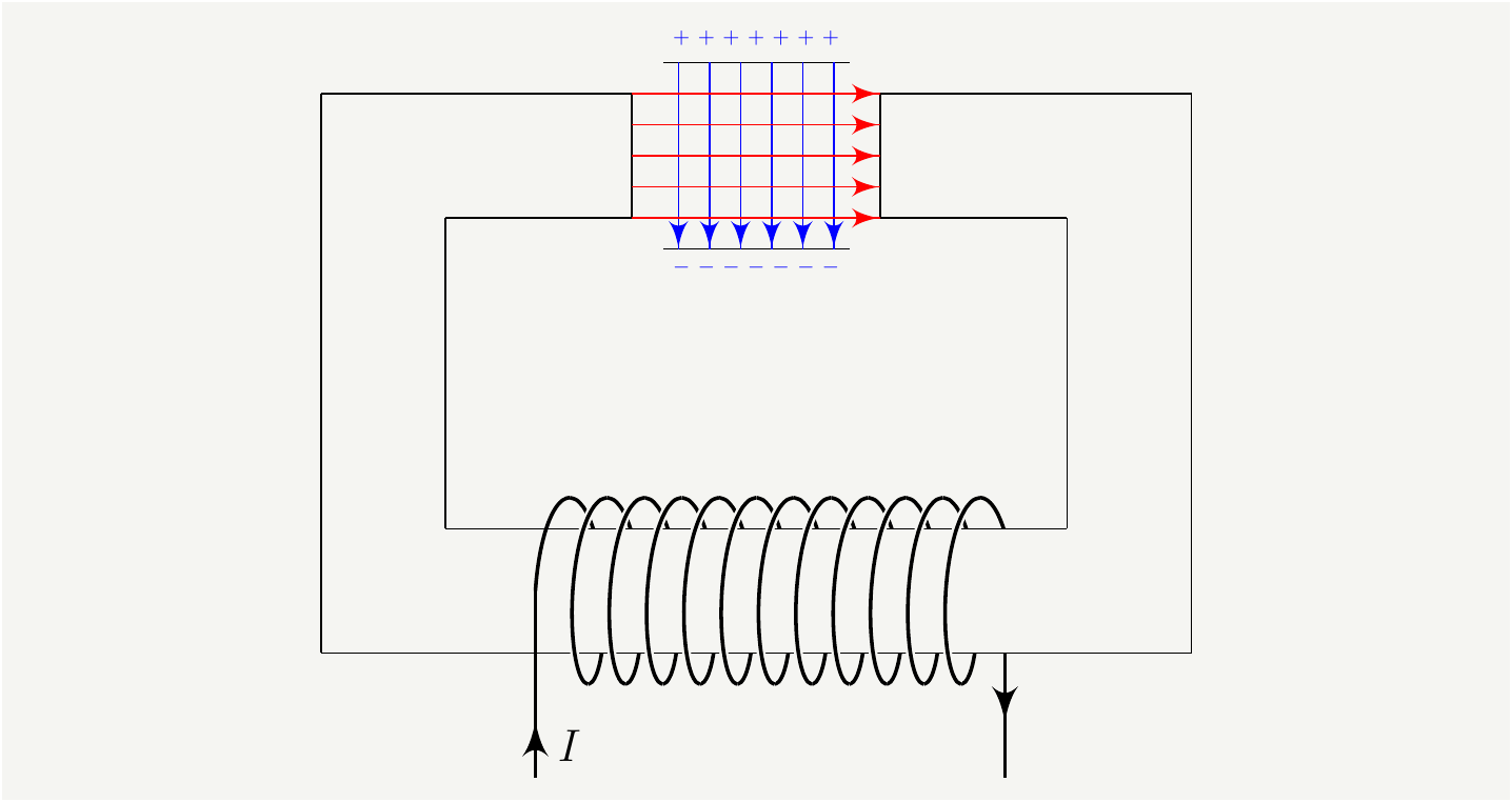
Figure 3: A setup with an electromagnet and a capacitor. Both electric and magnetic fields in the system are static. The are no moving charges between the capacitor plates. The electric and magnetic field lines are shown in blue and red, respectively.
Every single physical quantity in Fig. 3 is static. We could even remove the electromagnet with a permanent one and do away with the current. We are interested in figuring out what is going on inside the capacitor. As you may have predicted, nothing is happening there. No changing fields, no charges. It is as boring as it gets! The physical intuition says there is no energy flux whatsoever. But if you compute \(\mathbf S=\frac{1}{\mu_0}\mathbf {E}\times \mathbf B\) you find that it is non-zero, which would imply an energy flux. How come that be? A static electric field and a static magnetic field created by totally independent sources meeting at a point result in an energy flux? How did the math take us from a system that obviously has no flux to some apparent flux? You can trace that back to the step when we were looking into this object \(\mathbf {E} \cdot \mathbf {J}\) in the derivation of the Poynting theorem. Note here that \(\mathbf {J}=0\), so is \(\mathbf {E} \cdot \mathbf {J}=0\). Yet, we decided to replace \(\mathbf {J}\) with the fields (\(\mathbf {J}=\frac{1}{\mu_0}\mathbf{\nabla}\times\mathbf{B} -\varepsilon_0\frac{\partial\mathbf{E}}{\partial t}\)). What a strange thing to do: we replaced \(0\) with another \(0\). Did we break something?
Does it break conservation of energy?
Does this break physics and create an infinite energy source? Not really. The flux, if you insist to believe that it exists, is constant: it does not remove or add any energy. So we can still sleep at night without thinking that we have just broken the conservation of energy law.
Does it break conservation of momentum?
But, hold your horses! Maybe we have really broken a part of physics. Volume integral of \(\mathbf {S}\) is the total momentum carried by the EM field, and it is nonzero. Nothing is moving, yet there is momentum in the system! It is rather strange. It is not obvious if the conservation of momentum is violated or not. The momentum in the field might have been put in there as the fields were created. However, what happens if we turn the fields off by, say, discharging the capacitor or by reducing the current to zero slowly? At the end of the process, there will be no fields left, and the initial momentum in the fields has to go somewhere. As we are discharging the capacitor, there will be a current, and there will be a force induced by the magnetic field. Therefore, the capacitor will get a kick and acquire some momentum. However detailed analysis[6] shows that the total amount of momentum transferred to the capacitor is not equal to the original momentum in the fields. There seems to be some momentum hiding somewhere, or Poynting’s \(\mathbf {S}\) vector violates conservation of momentum. One can even build a space rocket out of it. This was introduced as a puzzle be Joseph Slepian[7] with the set up below.![A puzzle introduced Joseph Slepian: A setup that seemingly produces propulsion. Image taken from [@espace] and modified.](spr_r.png)
Figure 4: A puzzle introduced Joseph Slepian: A setup that seemingly produces propulsion. Image taken from [7] and modified.
You can see that if an alternating current is pushed through the wires it will create a changing magnetic field on the axis of the solenoid, which will also be accompanied by a circular electric field (Note the choice of words here: I am not saying changing magnetic field is inducing the electric field, because it doesn’t! See the last section.) That electric field will push the plates of the capacitor, and the push will be in the same direction as both the electric field and the charges flip signs at the opposite plates. So there seems to be a net force. However, it turns out that the mechanical momentum is equal in magnitude and opposite to the momentum in the field[8], therefore no net push! It is important to note that Slepian knew from the very beginning that this won’t produce net push, he introduced this as a pedagogical puzzle.
This doesn’t answer the question of the static capacitor discharging, though. If it exists, where is the hidden momentum?
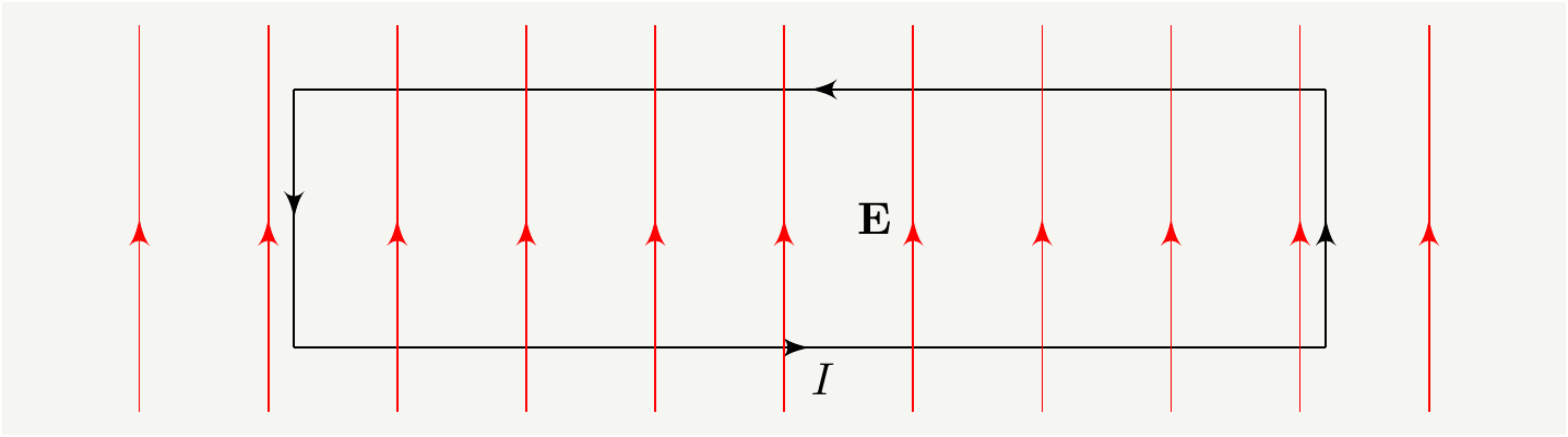
![A closer look at the current carrying loop inside the constant electric field. The current creates a magnetic field. The electric field accelerates the charges on the left wire and decelerates them on the right. Image reproduced from [@Babson2009HiddenMF].](https://tetraquark.netlify.app/post/energyflow/index_files/figure-html/loopc-1.png)
The real mechanism for energy transfer
We have shown that all the energy transfer on a circuit is facilitated only by the electric fields. What we have not discussed is how that electric field gets to the load in the first place. It is obvious in the case of static circuits: the source will re-arrange the charges on the wire so that the electric potential across the load is equal to that of the source. What we want to understand is how we get to the static case. Let’s us first understand how fast electrical fields move.
The speed
Consider the Maxwell’s equations away from the sources ( \(\mathbf {J}=0\) and \(\rho=0\)). Lets take \(\mathbf{\nabla}\times\) of Eq. (7): \[\begin{eqnarray} \mathbf{\nabla}\times( \mathbf{\nabla}\times\mathbf{E}) &=& -\frac{\partial }{\partial t}\left( \mathbf{\nabla}\mathbf\times{B}\right). \tag{31} \end{eqnarray}\] We need the following vector identity: \[\begin{eqnarray} \left(\mathbf{\nabla}\times[ \mathbf{\nabla}\times\mathbf{E}] \right)^i=\epsilon^{ijk}\epsilon^{klm}\partial_j\partial_l E_m =\left(\delta^{il}\delta^{jm}-\delta^{im}\delta^{jl}\right)\partial_j\partial_l E_m=\mathbf{\nabla}^i\left(\mathbf{\nabla}\cdot \mathbf{E}\right)-\mathbf{\nabla}^2 E^i. \tag{32} \end{eqnarray}\] Using the Ampere’s law from Eq. (8), we get \[\begin{eqnarray} \left( \mu_0\varepsilon_0 \frac{\partial^2}{\partial t^2}-\mathbf{\nabla}^2 \right)\mathbf{E}=0. \tag{33} \end{eqnarray}\] This is a wave equation with speed \(c=\frac{1}{\sqrt{\mu_0\varepsilon_0 }}\), which is the speed of light. This shows that any change in the electric fields will travel at the speed of light. If we really wanted, we could do the identical derivation for magnetic fields.
The vehicle
Assume the switch in Fig. 1 connected to the positive terminal of the battery is off. The load is connected to the negative terminal. At \(t=0\), you close the switch. And everyone tells you that the time it will take for the load to receive its first bit of power is \(d/c\), where \(d\) being the distance between the load and the source, and \(c\) is the speed of light. But, how? If you are a fan of the Poynting theorem, you will say, There is this \(\mathbf {S}\) vector that propagates at the speed of light, and it does that. And I ask again, how does it do that? I feel like I am repeating myself, but \(\mathbf {S}\) is not the ground truth here. It is an abstraction layer on top of the real process. Here is what really happens:
- As soon as the switch is closed, an electron is pulled from the wire to the positive terminal of the battery.
- Now that you have displaced an electron, its electric field moves a bit too.
- That disturbance propagates at the speed of light through space, see Eq. (33): the electric field is readjusting for the new position of the first electron.
- The shift is propagating in all directions, and it will reach to the load in \(d/c\) seconds.
- The electrons in the load and elsewhere will react to the changing field: they will actually move! Here you go, by displacing the electrons closest to the positive terminal of the battery, you delivered an electric field to the load (after \(d/c\) seconds of delay ).
- The charges in the load started moving as a response to this changing electric field: you got \(\mathbf {E} \cdot \mathbf{J}\), and it is non-zero. Congratulations, you just delivered power to your load.
- What has happened is this: An electron close to the load has responded to the change of the electric field of the electron that was close to the battery. So the energy is associated with the electric field, but the field itself is created by the electrons.
- As more electrons react to the switch being closed, they will rearrange themselves to create surface charges on the wires, which create a small gradient electric field in the wires slowly guiding electrons to the load and back.
You can say, “Hey, you moved some charges and moving charges create magnetic fields, what are you going to do about that?” And I will say, I will do nothing about it, it is just noise for energy transfer purposes. Sure, \(\mathbf {B}\) fields have energy because they exist, but that energy is not what the load gets.
This is the real mechanism to that delivers power from the source to load. Removing/adding electrons from/to the wire, the source propagates the energy in the electric field and that energy gets delivered to the load via the electrons.
I have to pick up on another thing Dr. Bruce Hunt says:People seem to think that you are pumping electrons and that you are buying electrons or something2, which is something so wrong.(laughs)…
So, although the professor laughs at it, this is exactly what the source does: it pumps electrons to create electric fields. That electric field extends to the load. Electrons, as they move under that field at the load, transfer energy to the LED or resistor. After they pass through the load, the source also slowly pulls them back and maintains the voltage difference. In alternating current, this simply switches direction 50-60 times per second. The source is still pumping and sucking the electrons back and forth through the load to deliver energy.
There is no mystery, no magnetic field, and no Poynting vector involved.
Solving Veritasium’s circuit analytically
Consider the circuit from the video as shown in Fig. 8, which extends half way to the moon. The bulb will get its first bit of energy in \(1m/c\) seconds. The mechanism we discussed above neatly explains why that is. As soon as a single electron moves when the switch is closed, its electric field will shift. And that change will propagate everywhere in the circuit. As that change arrives at the bulb, the electrons in the bulb will move creating a current and power. That is the whole story. Just ignore the magnetic fields, they are irrelevant.
Figure 8: A circuit that extends halfway to the moon. The load is only 1m away from the battery. Image taken from Veritasium video.
The power delivered to the bulb will increase with time as more and more electrons start reacting to the change. If the size of the circuit is similar to or larger than the wavelength of signals we are dealing with, things get interesting. Such large scale circuits are very important in power delivery systems and communication lines, and frequency response of such circuits can be readily found in engineering textbooks[15]. Time domain solutions are typically given by using so called bounce diagrams. Here I don’t want to rely on these diagrams. I want to derive the closed form solutions in time domain for a wide range of parameter space. Veritasium’s circuit is just one corner case of the full fledged solution. It is a tedious problem that requires certain knowledge of circuit theory, but it is not terribly complicated.
The telegrapher equations
It would be crazy to try to build a quantitative model of a circuit by keeping track of each and every charged particle and its fields. We have to simplify things. If you have taken any engineering classes, you will know how good engineers are in abstracting physical devices and lumping microscopic physics into more manageable objects. Can we explain the dynamics of signals propagating in a transmission line by using only the old-fashioned circuit theory? We sure can, and this topic is typically covered in engineering electromagnetism classes[15]. Let’s consider the circuit below which transmits signals (or power) from a source to a load over an abstracted transmission line.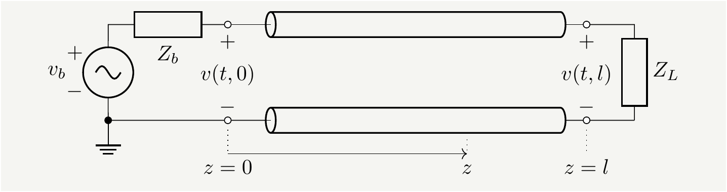
Figure 9: A source with an internal impedance of \(Z_b\) connected to a load via a transmission line. If you want to match elements of this circuit with Veritasium’s, \(Z_b\) would be the bulb, and \(Z_L=0\) as the circuit is shorted at the end. The switch that closes at \(t=0\) is not shown explicitly since it can be embedded in \(v_b(t)\).
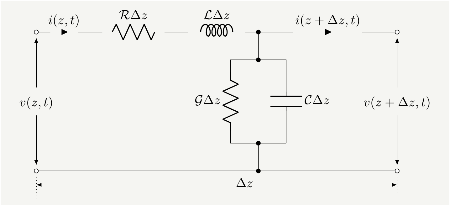
Figure 10: Equivalent circuit for a small piece of the transmission line. The paramaters, \(\mathcal{R}\), \(\mathcal{C}\), \(\mathcal{L}\), and \(\mathcal{G}\), are defined per unit length.
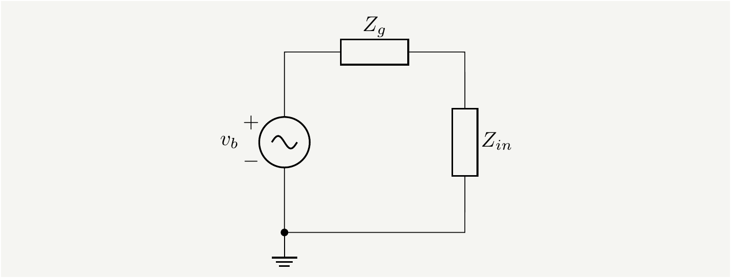
Figure 11: The transmission line and the load at the end of it are lumped into a single element \(Z_{in}\).
This is a simple voltage divider circuit and we can relate the voltage across \(Z_{in}\) to the source voltage \(v_b\) as as follows: \[\begin{eqnarray} v(z=0,t)=\frac{Z_{in}}{Z_{in}+Z_b} v_b(t) \quad \rightarrow \quad V(z=0,s)=\frac{Z_{in}}{Z_{in}+Z_b} V_b(s). \tag{48} \end{eqnarray}\] All we have to do now is to take \(Z_{in}\) from Eq. (46) and plug it in Eq. (48) and simplify the expression as follows: \[\begin{eqnarray} V(z=0,s)&=&\frac{Z_0\frac{ 1+\Gamma_L e^{-2\gamma l}}{ 1-\Gamma_L e^{-2\gamma l} }}{Z_0\frac{ 1+\Gamma_L e^{-2\gamma l}}{ 1-\Gamma_L e^{-2\gamma l} }+Z_b} V_b(s) =\frac{Z_0\left(1+\Gamma_L e^{-2\gamma l}\right)}{Z_0\left(1+\Gamma_L e^{-2\gamma l}\right)+Z_b\left(1-\Gamma_L e^{-2\gamma l}\right)} V_b(s)\nonumber\\ &=&\frac{Z_0\left(1+\Gamma_L e^{-2\gamma l}\right)}{Z_0+Z_j -(Z_0-Z_b)\Gamma_L} V_b(s)=\frac{Z_0}{Z_0+Z_b}\frac{1+\Gamma_L e^{-2\gamma l}}{1 -\Gamma_b\Gamma_L e^{-2\gamma l}} V_b(s), \tag{49} \end{eqnarray}\] where \(\Gamma_b\equiv\frac{Z_b-Z_0}{Z_0+Z_b}\) is the reflection coefficient on the battery side. But we also know that \(V(z=0,s)=V^++V^-=V^+\left(1+\frac{V^-}{V^-}\right)=\Gamma_L e^{-2\gamma l}\). We can now fix \(V^\pm\) as: \[\begin{eqnarray} V^+&=&\frac{Z_0}{Z_0+Z_b}\frac{1}{1 -\Gamma_b\Gamma_L e^{-2\gamma l}} V_b(s),\nonumber\\ V^-&=&\frac{Z_0}{Z_0+Z_b}\frac{\Gamma_L e^{-2\gamma l}}{1 -\Gamma_b\Gamma_L e^{-2\gamma l}} V_b(s). \tag{50} \end{eqnarray}\] We can finally write the voltage at the input of the transmission line as \[\begin{eqnarray} V(z,s)=V^- e^{\gamma z}+V^+ e^{-\gamma z}=V_b(s)\frac{Z_0}{Z_0+Z_b}\frac{1}{1 -\Gamma_b\Gamma_L e^{-2\gamma l}} \left(e^{-\gamma z}+\Gamma_L e^{\gamma( z-2 l)} \right). \tag{51} \end{eqnarray}\] All there is left to do is to invert this back to time domain. That is easier said than done due to various reasons. First of all, remember the nasty expressions: \(\gamma=\sqrt{(s\,\mathcal{L}+\mathcal{R})(s\,\mathcal{C}+\mathcal{G})}\), which sits in the exponents, and \(Z_0\equiv \sqrt{\frac{s\,\mathcal{L}+\mathcal{R} }{s\,\mathcal{C}+\mathcal{G}} }\) which appears everywhere. It is not possible to evaluate the inverse Laplace transform in a generic case. However, in the hypothetical lossless case, it will be a breeze. We can actually handle small resistance and small leakage case too. It is also important to remind ourselves that all \(Z\) and \(\Gamma\) terms in Eq. (51) could have \(s\) dependence if reactive elements are included, therefore we have to proceed carefully. Also note the denominator; how is that even possible to deal with that? It turns out that it is the exact term we didn’t know we needed!
Before we delve into more complicated cases, let’s warm up a bit by looking at a few interesting cases where impedances are perfectly or partially matched.
Perfectly matched circuit
Consider the case \(Z_b=Z_0=Z_L\) for which the reflection coefficients \(\Gamma_b=0=\Gamma_L\).The circuit will look like below.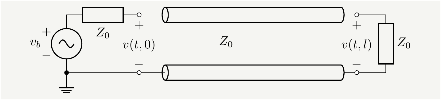
Figure 12: All the impedances are equal to each other:\(Z_L=Z_b=Z_0\). There will be no reflections in such a circuit.
Let us also assume that the circuit is lossless: \(\mathcal{R}=0=\mathcal{G}\), for which we have \(\gamma=s \sqrt{\mathcal{L}\mathcal{C}}\). Since it will appear so many times in our equations, it is convenient to define \(\frac{1}{\sqrt{\mathcal{L}\mathcal{C}}}\equiv c\), which is the speed of the waves. Putting this back into Eq. (51), we get \[\begin{eqnarray} V(z,s)&=&V_b(s)\cancelto{1/2}{\frac{Z_0}{Z_0+Z_b}}\frac{1}{1 -\cancelto{0}{\Gamma_b}\cancelto{0}{\Gamma_L} e^{-2\gamma l}} \left(e^{-\cancelto{\frac{s}{c} z}{\gamma z} }+\cancelto{0}{\Gamma_L} e^{\gamma( z-2 l)} \right)\nonumber\\ &=&\frac{1}{2} V_b(s)e^{-\frac{s}{c} z}, \tag{52} \end{eqnarray}\] and the corresponding time domain function down in the transmission line is simply \[\begin{eqnarray} v(z,t)=\mathscr{L}^{-1}\left[V(z,s)\right]&=&\frac{1}{2}v_b(t-\frac{z}{c}) U(t-\frac{z}{c}). \tag{53} \end{eqnarray}\] This shows that half of the source voltage is propagating to the right in the transmission line at the speed \(c\). Since the load impedance is matched, there will be no signal reflecting back. If we want to tie this to Veritasium’s circuit, we would be interested in the voltage across the bulb, which is represented by \(Z_b\) in our circuit: \[\begin{eqnarray} v_\text{bulb}(t)= v_b(t)-v(z=0,t)=\frac{1}{2}v_b(t) U(t), \tag{54} \end{eqnarray}\] which means that half of source voltage will appear across the bulb right after the switch is closed (with a delay of \(1m/c\)), and it will stay constant.
This was easy! We can actually do better than that with minimal effort. We want to include the effects of the resistance and the leakage at some lowest possible order. This will be a good approximation assuming that they are small to begin with, which ensures that higher order terms will be even smaller. Let’s turn on some small losses, \(\mathcal{R}, \mathcal{G}>0\), and expand \(\gamma\): \[\begin{eqnarray} \gamma&=&\sqrt{(s\,\mathcal{L}+\mathcal{R})(s\,\mathcal{C}+\mathcal{G})} =\sqrt{s^2\,\mathcal{L} \,\mathcal{C}+(\mathcal{G}+\mathcal{R})s+\mathcal{R}\mathcal{G}}=s\sqrt{\,\mathcal{L} \,\mathcal{C}}\sqrt{1+\frac{\mathcal{G}+\mathcal{R}}{\mathcal{L} \,\mathcal{C} s}+\frac{\mathcal{R}\mathcal{G}}{\mathcal{L} \,\mathcal{C} s^2} }\nonumber\\ &\simeq & s\sqrt{\,\mathcal{L} \,\mathcal{C}} + \frac{\mathcal{G}+\mathcal{R}}{2 \sqrt{\,\mathcal{L} \,\mathcal{C}}}= \frac{s}{c} +\zeta, \tag{55} \end{eqnarray}\] with \(\zeta\equiv \frac{\mathcal{G}+\mathcal{R}}{2 \sqrt{\,\mathcal{L} \,\mathcal{C}}}\). Putting this back into Eq. (51) again, we get \[\begin{eqnarray} V(z,s)&=&\frac{1}{2} V_b(s)e^{-\frac{s}{c} z -\zeta z}, \tag{56} \end{eqnarray}\] and the corresponding time domain function down in the transmission line is simply \[\begin{eqnarray} v(z,t)=\mathscr{L}^{-1}\left[V(z,s)\right]&=&\frac{1}{2}e^{-\zeta z}v_b(t-\frac{z}{c}) U(t-\frac{z}{c}). \tag{57} \end{eqnarray}\] This now shows that the signal will decay exponentially as it propagates through the line. Note that this doesn’t bother the voltage on \(Z_b\), i.e., the bulb, since all it sees is \(v(z=0,t)\). So the bulb wouldn’t care if the line is lossy or not in the perfectly matched case.
Half matched circuit
Consider the case \(Z_b=Z_0\neq Z_L\) for which the reflection coefficients \(\Gamma_b=0\neq\Gamma_L\), and a transmission line with small losses: \(\gamma=\frac{s}{c} +\zeta\). The circuit looks like below: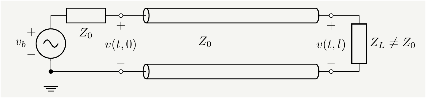
Figure 13: The internal impedance of the battery is matched with the characteristic impedance of the line: \(Z_b=Z_0\). Since load impedance \(Z_L\) is different than \(Z_0\), we expect waves reflecting back from the end of the line.
Putting the reflection coefficients back into Eq. (51), we get \[\begin{eqnarray} V(z,s)&=&V_b(s)\cancelto{1/2}{\frac{Z_0}{Z_0+Z_b}}\frac{1}{1 -\cancelto{0}{\Gamma_b}\Gamma_L e^{-2\gamma l}} \left( e^{-\cancelto{(\frac{s}{c}+\zeta)z}{\gamma z} }+\Gamma_L e^{\cancelto{(\frac{s}{c}+\zeta)}{\gamma z}( z-2 l)} \right)\nonumber\\ &=&V_b(s)\frac{1}{2} \left( e^{-(\frac{s}{c}+\zeta)z }+\Gamma_L e^{(\frac{s}{c}+\zeta)( z-2 l)} \right) \tag{58} \end{eqnarray}\] Assuming \(Z\)’s have no \(s\) dependence in them, the corresponding time domain function down in the transmission line is \[\begin{eqnarray} v(z,t)=\mathscr{L}^{-1}\left[V(z,s)\right]&=&\frac{1}{2} e^{-\zeta z} v_b(t-\frac{z}{c}) U(t-\frac{z}{c})+\frac{\Gamma_L}{2} e^{-(2l-z) \zeta } v_b(t-\frac{2 l-z}{c}) U(t-\frac{2l-z}{c}), \tag{59} \end{eqnarray}\] which is a combination of two waves propagating in the opposite directions. As the reflected wave hits back to the source side, that’s the end of the dynamics: there is no reflection from the source back to the line. Let us take a quick look at the cases of open and short circuit lines.
Open circuit at the end
That is \(Z_L\to \infty\), which means \(\Gamma_L=\frac{ Z_L-Z_0} { Z_L+Z_0 }\to 1\), and the voltage across the transmission line becomes: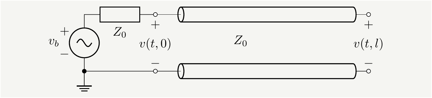
Figure 14: The internal impedance of the battery is matched with the characteristic impedance of the line: \(Z_b=Z_0\). Since load impedance \(Z_L\to \infty\), it will reflect all signals with \(\Gamma_L=1\).
\[\begin{eqnarray} v(z,t)&=&\frac{1}{2} e^{-\zeta z} v_b(t-\frac{z}{c}) U(t-\frac{z}{c})+\frac{1}{2} e^{-(2l-z) \zeta } v_b(t-\frac{2 l-z}{c}) U(t-\frac{2l-z}{c}). \tag{60} \end{eqnarray}\] If \(\zeta=0\) (no loss in the line): \[\begin{eqnarray} v(z,t)&=&\frac{1}{2} v_b(t-\frac{z}{c}) U(t-\frac{z}{c})+\frac{1}{2} v_b(t-\frac{2 l-z}{c}) U(t-\frac{2l-z}{c}). \tag{61} \end{eqnarray}\] We see that \(v(z=0,t<\frac{2l}{c})=\frac{1}{2} v_b(t)\): the voltage at the input of the line (\(z=0\)) is half of the source voltage. This means \(Z_b\), the bulb, will have \(v_\text{bulb}(t<\frac{2l}{c})=\frac{1}{2} v_b(t)\), that is half of the source voltage. After \(t>\frac{2l}{c}\), the reflected wave comes back and adds the same amount of voltage to give: \(v(z=0,t>\frac{2l}{c})= v_b(t)\) at the input terminal of the line. Now the bulb voltage will drop to \(0\), and it will turn off- it is connected to an open circuit anyways! Isn’t this awesome?
If \(\zeta>0\) (small losses in the line), \(v(z=0,t<\frac{2l}{c})=\frac{1}{2} v_b(t)\). After \(t>\frac{2l}{c}\), the reflected wave comes back and adds \(\frac{1}{2} e^{-2l \zeta } v_b(t-\frac{2 l}{c})\) at \(z=0\), which is probably a very small amount due to the \(e^{-2l \zeta }\) term. If we ignore the contribution from the reflected wave, we can say \(v(z=0,t)=\frac{1}{2} v_b(t)\), that is constant at the half value of the source voltage. This shows that the bulb will also get half: \(v_\text{bulb}(t)=\frac{1}{2} v_b(t)\). Is this strange? The circuit is open on the other end, but the bulb will always get half of the source voltage no matter how long we wait. Did we break something? Nope, the transmission line is leaky. It is still drawing current since it is not lossless. It is effectively a resistor of value \(Z_b\), so voltage is equally split between the line and the bulb.
Short circuit at the end
Here we have \(Z_L\to 0\), which means \(\Gamma_L=\frac{ Z_L-Z_0} { Z_L+Z_0 }\to -1\). The circuit is shown below.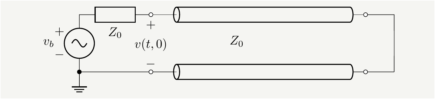
Figure 15: The internal impedance of the battery is matched with the characteristic impedance of the line: \(Z_b=Z_0\). Since load impedance \(Z_L=0\), it will reflect all signals with \(\Gamma_L=-1\).
The voltage across the transmission line becomes: \[\begin{eqnarray} v(z,t)&=&\frac{1}{2} e^{-\zeta z} v_b(t-\frac{z}{c}) U(t-\frac{z}{c})-\frac{1}{2} e^{-(2l-z) \zeta } v_b(t-\frac{2 l-z}{c}) U(t-\frac{2l-z}{c}). \tag{62} \end{eqnarray}\] If \(\zeta=0\) (no loss in the line): \[\begin{eqnarray} v(z,t)&=&\frac{1}{2} v_b(t-\frac{z}{c}) U(t-\frac{z}{c})-\frac{1}{2} v_b(t-\frac{2 l-z}{c}) U(t-\frac{2l-z}{c}). \tag{63} \end{eqnarray}\] We observe that \(v(z=0,t<\frac{2l}{c})=\frac{1}{2} v_b(t)\): the voltage at the input of the line (\(z=0\)) is half of the source voltage. This means \(Z_b\), the bulb, will \(v_\text{bulb}(t<\frac{2l}{c})=\frac{1}{2} v_b(t)\). After \(t>\frac{2l}{c}\), the reflected wave comes back and subtracts the same amount of voltage to give: \(v(z=0,t>\frac{2l}{c})= 0\). The bulb voltage will rise to \(v_b\)- it is connected to a short circuit anyways!
If \(\zeta>0\) (small losses in the line), \(v(z=0,t<\frac{2l}{c})=\frac{1}{2} v_b(t)\). After \(t>\frac{2l}{c}\), the reflected wave comes back and adds \(\frac{1}{2} e^{-2l \zeta } v_b(t-\frac{2 l}{c})\) at \(z=0\), which is again probably a very small number. So the bulb voltage will remain the same. It won’t notice the difference between short vs open ends if there is too much loss on the way.
Reactive loads
Are You Not Entertained? Resistive loads are almost boring, don’t you think? They reflect the incoming signal after scaling it down with a possible polarity flip. They don’t really change the shape of the signal. Let’s spice things up a bit. What happens if \(Z_L\) has some reactive components, capacitors or inductors or a diode? In such cases \(Z_L\) is \(s\) dependent, so is \(\Gamma_L\). Remember that, when \(\Gamma_b=0\), for the reflections we have to compute this: \[\begin{eqnarray} e^{-\zeta( 2 l-z)} \mathscr{L}^{-1}\left[\Gamma_L(s) V_b(s) e^{\frac{s}{c}( z-2 l)} \right]=e^{-\zeta( 2 l-z)} \left(\gamma_L *v_b\right)(t-\frac{z-2 l}{c}), \tag{64} \end{eqnarray}\] where \(*\) denotes the convolution integral, and \(\gamma_L(t)\) is defined as follows: \[\begin{eqnarray} \gamma_L(t)\equiv\mathscr{L}^{-1}\left[\Gamma_L\right]. \tag{65} \end{eqnarray}\] This result is based on the convolution and shift properties of Laplace transforms. As a sanity check, we can try to confirm that we can reproduce earlier results in which \(\Gamma_L=\pm 1\). For those cases \(\gamma_L(t)=\mathscr{L}^{-1}\left[\Gamma_L\right]=\pm \delta(t)\), where \(\delta(t)\) is the Dirac-delta function. We know that \(\left(\delta *v_b\right)(t)=v_b(t)\), hence the function is reflected unchanged up to its sign. Let’s now consider a reactive load composed of an inductor \(L\) and a resistor \(R\) in series, as illustrated below:
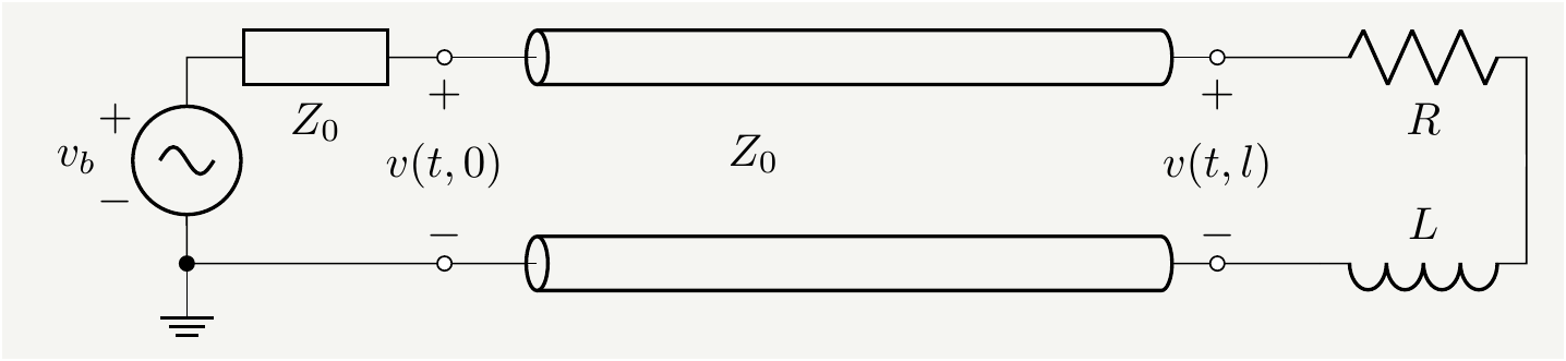
Figure 16: The internal impedance of the battery is matched with the characteristic impedance of the line: \(Z_b=Z_0\). The load is an inductor in series with a resistor.
The load impedance becomes: \[\begin{eqnarray} Z_L(s)&=&R+Ls. \tag{66} \end{eqnarray}\] The reflection coefficient becomes: \[\begin{eqnarray} \Gamma_L(s)=\frac{ Z_L-Z_0} { Z_L+Z_0 }=1-\frac{ 2Z_0} { Z_L+Z_0 }=1-\frac{ 2Z_0} { Ls +R +Z_0 }=1-\frac{ \frac{2 Z_0}{L}} {s +\frac{R +Z_0}{L} }. \tag{67} \end{eqnarray}\] The time domain function is: \[\begin{eqnarray} \gamma_L(t)=\mathscr{L}^{-1}\left[\Gamma_L\right]=\left(\delta(t)- \frac{2 Z_0}{L}e^{-t\frac{R +Z_0}{L} }\right)U(t). \tag{68} \end{eqnarray}\] We just need to convolve it with \(v_b(t)\): \[\begin{eqnarray} \left(\gamma_L *v_b\right)(t)&=&\int_{-\infty}^{\infty} d\tau \gamma_L (\tau)v_b(t-\tau)=\int_{-\infty}^{\infty} d\tau \left(\delta(\tau)- \frac{2 Z_0}{L}e^{-\tau\frac{R +Z_0}{L} }\right)U(\tau)v_b(t-\tau)\nonumber\\ &=&v_b(t)- \frac{2 Z_0}{L}\int_{0}^{\infty} d\tau e^{-\tau\frac{R +Z_0}{L} }v_b(t-\tau). \tag{69} \end{eqnarray}\] If the source signal is constant for \(t>0\), we have \(v_b(t)=V U(t)\), and the convolution becomes: \[\begin{eqnarray} \left(\gamma_L *v_b\right)(t)=V U(t)- \frac{2 V Z_0}{L}\int_{0}^{t} d\tau e^{-\tau\frac{R +Z_0}{L} }=V U(t)\left(\frac{R-Z_0}{R+Z_0}+ \frac{2 Z_0}{R+Z_0}e^{-t\frac{R +Z_0}{L} }\right). \tag{70} \end{eqnarray}\] The full expression for the voltage on the line becomes: \[\begin{eqnarray} v(z,t)=\frac{V}{2} e^{-\zeta z} U(t-\frac{z}{c})+\frac{V}{2} e^{-(2l-z) \zeta } \left( \frac{R-Z_0}{R+Z_0}+ \frac{2 Z_0}{R+Z_0}e^{-\left[t-\frac{2 l-z}{c}\right]\frac{R +Z_0}{L} } \right) U(t-\frac{2l-z}{c}). \tag{71} \end{eqnarray}\] We could go through the same exercise for other reactive loads. It all comes down to calculating \(\left(\gamma_L *v_b\right)(t)\) and reflecting it back.
Turtles all the way up and down

Figure 17: The main signal at the input terminals of a mismatched transmission line will have its reflections as it reaches to the end of the line. The reflections will travel back only to reflect back again. It is just scaled reflections all the way up and down. Image credit: Wikipedia.
Let us consider the case of completely mismatched impedances. We still assume that the losses on the transmission line is small: \(\gamma=s/c+\zeta\) as in Eq. (55). And to avoid multiple convolution integrals, we will assume that none of the \(Z\)’s has \(s\) dependence at the order we are interested. We have to verify this assumption for \(Z_0\) by expanding it carefully: \[\begin{eqnarray} Z_0=\sqrt{\frac{s\,\mathcal{L}+\mathcal{R} }{s\,\mathcal{C}+\mathcal{G}} } =\sqrt{\mathcal{L} \,\mathcal{C} }\sqrt{1+\frac{\mathcal{G}+\mathcal{R}}{\,\mathcal{L} \,\mathcal{C} s}+ \frac{\mathcal{G}\mathcal{R}}{\,\mathcal{L} \,\mathcal{C} s^2} }\simeq \sqrt{\mathcal{L} \,\mathcal{C} }+\mathcal{O}(1/s), \tag{72} \end{eqnarray}\] which means that we can treat the impedance of the transmission line as a resistor at the first order. This makes the exponentials in the numerator very easy to handle since they will be simple time shifts or scales. We can do the following trick to get rid of the denominator: \[\begin{eqnarray} \frac{1}{1 -\Gamma_b\Gamma_L e^{-2\gamma l}}=\sum_{k=0}^\infty \left(\Gamma_b\Gamma_L\right)^k e^{-2\gamma l k}=\sum_{k=0}^\infty \left(\Gamma_b\Gamma_L\right)^k e^{-2 lk (\frac{s}{c}+\zeta) } \tag{73}. \end{eqnarray}\] We can then insert this expansion back into Eq. (51) and evaluate the inverse Laplace transform: \[\begin{eqnarray} v(z,t)&=&\mathscr{L}^{-1}\left[V(z,s)\right]=\frac{Z_0}{Z_0+Z_b}\sum_{k=0}^\infty \left(\Gamma_b\Gamma_L\right)^k \mathscr{L}^{-1}\left[ V_b(s)\left( e^{-2 lk (\frac{s}{c}+\zeta) - (\frac{s}{c}+\zeta)z } +\Gamma_L e^{-2 lk (\frac{s}{c}+\zeta) + (\frac{s}{c}+\zeta) (z-2 l) } \right) \right] \nonumber\\ &=&\frac{Z_0}{Z_0+Z_b}\sum_{k=0}^\infty \left(\Gamma_b\Gamma_L\right)^k\left[ v_b\left(t- \frac{2 k l -z}{c} \right)U\left(t- \frac{2 k l -z}{c} \right) e^{-(2 lk+z) \zeta } \right. \nonumber\\ && \quad\quad\quad \quad\quad\quad \quad\quad\quad \quad +\left. \Gamma_L v_b\left(t+ \frac{z-2 (k+1) l}{c}\right) U\left(t+ \frac{z-2 (k+1) l}{c}\right) e^{-(2 l(k+1)-z) \zeta } \right]. \tag{74} \end{eqnarray}\] This is the most general equation excluding the case of reactive elements. Let’s entertain certain corner cases.
Short circuit at the end
Let us revisit the line short circuited at the end: \(Z_L= 0\). This is very close3 to the circuit in the video. This means \(\Gamma_L=\frac{ Z_L-Z_0} { Z_L+Z_0 }= -1\), and the voltage across the transmission line becomes: \[\begin{eqnarray} v(z,t)&=&\frac{Z_0}{Z_0+Z_b}\sum_{k=0}^\infty \left(-\Gamma_b\right)^k\left[ v_b\left(t- \frac{2 k l -z}{c} \right)U\left(t- \frac{2 k l -z}{c} \right) e^{-(2 lk+z) \zeta } \right. \nonumber\\ && \quad\quad\quad \quad\quad\quad \quad\quad\quad \quad -\left. v_b\left(t+ \frac{z-2 (k+1) l}{c}\right) U\left(t+ \frac{z-2 (k+1) l}{c}\right) e^{-(2 l(k+1)-z) \zeta } \right]. \tag{75} \end{eqnarray}\] In the spirit of pushing things further analytically, let’s assume a constant battery voltage turning on at \(t=0\), i.e., \(v_g(t)=VU(t)\), and check what is going on at the input terminal of the transmission line (\(z=0\)): \[\begin{eqnarray} v(z=0,t)&=&\frac{V Z_0}{Z_0+Z_b}\sum_{k=0}^\infty \left(-\Gamma_b\right)^k\left[ U\left(t- \frac{2 k l}{c} \right)e^{-2 lk \zeta } - U\left(t -\frac{2 (k+1) l}{c}\right) e^{-2 l(k+1) \zeta } \right]. \tag{76} \end{eqnarray}\] One thing we notice immediately is that if \(t\) is large, unitstep functions will cancel each other until some large \(k^*\) in the summation. Indices larger than \(k^*\) will be suppressed by \(\left(-\Gamma_b\right)^k e^{-2 lk \zeta }\), so they won’t contribute much. This means the voltage will converge to \(0\) for large \(t\). If you want to make sense of the expression, you can explicitly write down the terms for \(k=0,1,\cdots\). I want to get to a closed form expression, though. We have to chug along. Consider the summation over the first step function, and notice that the step function simply truncates the summation at \(k=\lfloor{\frac{t c}{2 l}}\rfloor\), where \(\lfloor\, \rfloor\) denotes the flooring operation. We then have the following summation to evaluate:
\[\begin{eqnarray} S_1&\equiv&\sum_{k=0}^\infty \left(-\Gamma_b\right)^k U\left(t- \frac{2 k l}{c} \right)e^{-2 lk \zeta } =\sum_{k=0}^{ \lfloor\frac{t c}{2 l} \rfloor} \left(-\Gamma_b e^{-2 l \zeta }\right)^k =\frac{1-\left(-\Gamma_b e^{-2 l \zeta }\right)^{1+\lfloor{\frac{t c}{2 l}}\rfloor} }{1+\Gamma_b e^{-2 l \zeta }}. \tag{77} \end{eqnarray}\]
The second summation is very similar. We just need to shift the summation index properly: \[\begin{eqnarray} S_2&\equiv&\sum_{k=0}^\infty \left(-\Gamma_b\right)^k U\left(t -\frac{2 (k+1) l}{c}\right) e^{-2 l(k+1) \zeta } =e^{-2 l \zeta }\sum_{k=0}^{\lfloor\frac{t c}{2 l} \rfloor -1} \left(-\Gamma_b e^{-2 l \zeta }\right)^k =e^{-2 l \zeta }\frac{1-\left(-\Gamma_b e^{-2 l \zeta }\right)^{\lfloor{\frac{t c}{2 l}}\rfloor} }{1+\Gamma_b e^{-2 l \zeta }}. \tag{78} \end{eqnarray}\] Combined together they give:
\[\begin{eqnarray} v(z=0,t)&=&\frac{V Z_0}{Z_0+Z_b}\left(S_1-S_2 \right)= \frac{VZ_0}{Z_0+Z_b}\left(\frac{1-\left(-\Gamma_b e^{-2 l \zeta }\right)^{1+\lfloor{\frac{t c}{2 l}}\rfloor} }{1+\Gamma_b e^{-2 l \zeta }} -e^{-2 l \zeta }\frac{1-\left(-\Gamma_b e^{-2 l \zeta }\right)^{\lfloor{\frac{t c}{2 l}}\rfloor} }{1+\Gamma_b e^{-2 l \zeta }} \right). \tag{79} \end{eqnarray}\] Let’s see if this simplifies for \(\zeta=0\): \[\begin{eqnarray} v(z=0,t)&=& \frac{V Z_0}{Z_0+Z_b}\left(\frac{\left(-\Gamma_b\right)^{\lfloor{\frac{t c}{2 l}}\rfloor}-\left(-\Gamma_b\right)^{1+\lfloor{\frac{t c}{2 l}}\rfloor} }{1+\Gamma_b } \right)=\frac{V Z_0}{Z_0+Z_b} \left(-\Gamma_b\right)^{\lfloor{\frac{t c}{2 l}}\rfloor}= \frac{V Z_0}{Z_0+Z_b}\left(\frac{Z_0-Z_b}{Z_0+Z_b}\right)^{\lfloor{\frac{t c}{2 l}}\rfloor} \tag{80}. \end{eqnarray}\] This is kind of interesting. Since \(\left|\frac{Z_0-Z_b}{Z_0+Z_b}\right|<1\), this tells us that the voltage at the input of the transmission line will decay in absolute value over time. But it will be a wild ride if \(Z_b>Z_0\): we will be taking integer powers of a negative number, and the result will swing from positive negative! This makes sense. The reflection from the end terminal returns the signal with a negative sign (\(\Gamma_L=-1\)). As it is returning, it is erasing the signal propagating to the right. It comes back to the battery, reflects again, without flipping (\(\Gamma_b>0\)), now it is moving to the right erasing even more of the signal, so much so that it can flip its sign! All of these behaviors are captured in our neat formula! The stepwise nature of the function is encapsulated in the \(\lfloor\, \rfloor\) operator. If we are interested in the voltage across the bulb, which is represented by \(Z_b\), it is simply the following:
\[\begin{eqnarray} v_\text{bulb}(t)=V- v(z=0,t)= V- \frac{V Z_0}{Z_0+Z_b}\left(\frac{Z_0-Z_b}{Z_0+Z_b}\right)^{\lfloor{\frac{t c}{2 l}}\rfloor} \tag{81}. \end{eqnarray}\] It starts from \(\frac{V Z_b}{Z_0+Z_b}\) and climbs up to \(V\). We can compare the prediction from this equation against one of the simulations done by Richard Abbott of Caltech[16]. He has a plot for \(Z_0=20\times Z_\text{bulb}\) (Note that there is a factor of \(2\) difference in my definition of \(Z_0\) vs his since I am looking at half of the circuit due to the symmetry. So, in my formula \(Z_0=10\times Z_\text{bulb}\)). I don’t have access to the data behind the plot, but I can overlay my formula on top of the image using some simple Python image processing.
  # Fitting a voltage curve on plot image
  #  12/29/2021, tetraquark@gmail.com
  # https://tetraquark.netlify.app/post/energyflow/#Turtlesallthewayupanddown

  from PIL import Image
  import math

  imgPath=""
  imgid= 'abbott.png' # taken from https://docs.google.com/presentation/d/1onHMsDkEARxagluUmHHS2as6YPWWAyDO/edit?rtpof=true&sd=true

  img = Image.open(imgPath+imgid)

  pixels = img.load()
  #calibrate these values to match the origin, xrange and aspect ratio
  cx=60
  cy=img.size[1]-56
  tdivider=20   # number of seconds on the t-axis
  xrange=  945
  tscale=(xrange)/tdivider
  aspectR=0.746


  Z0=20    # characteristic impedance
  Zs=2     # impedance of the bulb
  c1=Z0/(Z0+Zs)
  c2=(Z0-Zs)/(Z0+Zs)

  def v(x):
      tv=(x -cx)/tscale
      tv=  math.floor(tv)
      vv=   cy-aspectR*xrange*(1-c1*c2**tv)
      return  vv

  for i in range(cx,cx+xrange):
      for j in range(3):
              h=  v(i)+j
              if 1<h< img.size[1]:
               pixels[i,h ] = (0, 0,255)
  #img.show()
  img.save('marked_'+imgid)
Figure 18: The blue line shows the predicted voltage across the bulb, overlayed on top of the simulation plot from Richard Abbott. Ignore the red line since it is for another case.
It is a perfect match which gives us a bit more confidence that we are on the right track.
Open circuit at the end
Let us rinse and repeat for a transmission line with an open circuit at the end: \(Z_L\to \infty\). This means \(\Gamma_L=\frac{ Z_L-Z_0} { Z_L+Z_0 }= 1\), and the voltage across the transmission line becomes: \[\begin{eqnarray} v(z,t)&=&\frac{Z_0}{Z_0+Z_b}\sum_{k=0}^\infty \left(\Gamma_b\right)^k\left[ v_b\left(t- \frac{2 k l -z}{c} \right)U\left(t- \frac{2 k l -z}{c} \right) e^{-(2 lk+z) \zeta } \right. \nonumber\\ && \quad\quad\quad \quad\quad\quad \quad\quad\quad \quad +\left. v_b\left(t+ \frac{z-2 (k+1) l}{c}\right) U\left(t+ \frac{z-2 (k+1) l}{c}\right) e^{-(2 l(k+1)-z) \zeta } \right]. \tag{82} \end{eqnarray}\]
Assume again a constant battery voltage turning on at \(t=0\), i.e., \(v_g(t)=VU(t)\), and check what is going on at the input terminal of the transmission line (\(z=0\)): \[\begin{eqnarray} v(z=0,t)&=&\frac{V Z_0}{Z_0+Z_b}\sum_{k=0}^\infty \left(\Gamma_b\right)^k\left[ U\left(t- \frac{2 k l}{c} \right)e^{-2 lk \zeta } + U\left(t -\frac{2 (k+1) l}{c}\right) e^{-2 l(k+1) \zeta } \right]. \tag{83} \end{eqnarray}\] We go through the same steps with the sign flip to get \[\begin{eqnarray} v(z=0,t)&=&\frac{V Z_0}{Z_0+Z_b}\left(S_1+S_2 \right)= \frac{V Z_0}{Z_0+Z_b}\left(\frac{1-\left(\Gamma_b e^{-2 l \zeta }\right)^{1+\lfloor{\frac{t c}{2 l}}\rfloor} }{1-\Gamma_b e^{-2 l \zeta }} +e^{-2 l \zeta }\frac{1-\left(\Gamma_b e^{-2 l \zeta }\right)^{\lfloor{\frac{t c}{2 l}}\rfloor} }{1-\Gamma_b e^{-2 l \zeta }} \right). \tag{84} \end{eqnarray}\] Simplifying for \(\zeta=0\): \[\begin{eqnarray} v(z=0,t)&=& \frac{V Z_0}{Z_0+Z_b}\left(\frac{2-\left(\Gamma_b\right)^{\lfloor{\frac{t c}{2 l}}\rfloor}-\left(\Gamma_b\right)^{1+\lfloor{\frac{t c}{2 l}}\rfloor} }{1-\Gamma_b } \right)=\frac{V Z_0}{Z_0+Z_b} \left(\frac{2-\left(\Gamma_b\right)^{\lfloor{\frac{t c}{2 l}}\rfloor}(1+\Gamma_b) }{1-\Gamma_b } \right). \tag{85}. \end{eqnarray}\] Let’s first compute the overall factor for the constant term, \[\begin{eqnarray} \frac{ V Z_0}{Z_0+Z_b}\frac{1}{1-\Gamma_b }=\frac{V}{2} \tag{86}, \end{eqnarray}\] and the overall factor for the time dependent term, \[\begin{eqnarray} \frac{ V Z_0}{Z_0+Z_b}\frac{1+\Gamma_b}{1-\Gamma_b }=\frac{V Z_b}{Z_0+Z_b} \tag{87}, \end{eqnarray}\] and put them back in: \[\begin{eqnarray} v(z=0,t)&=&V- \frac{V Z_b}{Z_0+Z_b}\left(\Gamma_b\right)^{\lfloor{\frac{t c}{2 l}}\rfloor} =V- \frac{V Z_b}{Z_0+Z_b}\left( \frac{ Z_b-Z_0} { Z_b+Z_0 } \right)^{\lfloor{\frac{t c}{2 l}}\rfloor}. \tag{88} \end{eqnarray}\]
This tells us that the voltage at the input of the transmission line will start from \(\frac{V Z_0}{Z_0+Z_b}\) and grow to \(V\) stepwise as waves travel back to the input terminal. If we are interested in the voltage across the bulb, which is represented by \(Z_b\), it is simply the following:
\[\begin{eqnarray} v_\text{bulb}(t)=V- v(z=0,t)=\frac{V Z_b}{Z_0+Z_b}\left( \frac{ Z_b-Z_0} { Z_b+Z_0 } \right)^{\lfloor{\frac{t c}{2 l}}\rfloor} \tag{89}. \end{eqnarray}\] It starts from \(\frac{V Z_b}{Z_0+Z_b}\) and decays to \(0\). Also note the interesting behavior for \(Z_b<Z_0\). As we discussed earlier, the voltage will swing back and forth from positive to negative before it settles to \(0\).
One formula to rule them all
We have been looking at various the corner cases, because I didn’t think the problem would be solvable in a closed form for generic values of \(Z_b\), \(Z_L\) relative to \(Z_0\). This has been a learning process for me too, and the exercises I have gone through give me the confidence that we can evaluate Eq. (74) in closed form if we proceed carefully. We would like to be able to recover the cases with \(\Gamma_L\to 0\) and \(\Gamma_b\to 0\), and all of that information is at the \(k=0\) term in the summations. To avoid \(0^0\) ambiguity, we can say we will evaluate the summation first then take the \(\Gamma_L\to 0\) and \(\Gamma_b\to 0\) limits. That should reproduce our earlier results. Let’s evaluate the first summation: \[\begin{eqnarray} S_1 &=&\sum_{k=0}^\infty \left(\Gamma_b\Gamma_L e^{-2 l\zeta }\right)^k v_b\left(t- \frac{2 k l -z}{c} \right)U\left(t- \frac{2 k l -z}{c} \right) e^{-(2 l(k+1)-z) \zeta } \nonumber\\ &=&e^{-\zeta z } \sum_{k=0}^{\lfloor{\frac{t c+z}{2 l}}\rfloor} \left(\Gamma_b\Gamma_L e^{-2 l\zeta }\right)^k = e^{-\zeta z }\frac{1-\left(\Gamma_L\Gamma_b e^{-2 l \zeta }\right)^{1+\lfloor{\frac{t c +z}{2 l}}\rfloor} }{1-\Gamma_L \Gamma_b e^{-2 l \zeta }}, \tag{90} \end{eqnarray}\] and the second: \[\begin{eqnarray} S_2 &=&\sum_{k=0}^\infty \left(\Gamma_b\Gamma_L\right)^k \Gamma_L v_b\left(t+ \frac{z-2 (k+1) l}{c}\right) U\left(t+ \frac{z-2 (k+1) l}{c}\right) e^{-(2 l(k+1)-z) \zeta } \nonumber\\ &=& e^{-(2 l-z) \zeta } \Gamma_L \sum_{k=0}^{\lfloor{\frac{t c-z}{2 l}}\rfloor-1}\left(\Gamma_b\Gamma_L e^{-2 l \zeta }\right)^k = e^{-(2 l-z) \zeta } \Gamma_L \frac{1-\left(\Gamma_L\Gamma_b e^{-2 l \zeta }\right)^{\lfloor{\frac{t c -z}{2 l}}\rfloor} }{1-\Gamma_L \Gamma_b e^{-2 l \zeta }}. \tag{91} \end{eqnarray}\] Combining them, we get: \[\begin{eqnarray} v(z,t)&=&\frac{V Z_0}{Z_0+Z_b}\left(S_1+S_2 \right)= \frac{V Z_0}{Z_0+Z_b} \left[ e^{-\zeta z }\frac{1-\left(\Gamma_L\Gamma_b e^{-2 l \zeta }\right)^{1+\lfloor{\frac{t c +z}{2 l}}\rfloor} }{1-\Gamma_L \Gamma_b e^{-2 l \zeta }} + e^{-(2 l-z) \zeta } \Gamma_L \frac{1-\left(\Gamma_L\Gamma_b e^{-2 l \zeta }\right)^{\lfloor{\frac{t c -z}{2 l}}\rfloor} }{1-\Gamma_L \Gamma_b e^{-2 l \zeta }}\right]. \tag{92} \end{eqnarray}\] We can throw anything, except for reactive loads, at this equation, and it will work. Also, just an observation: the effect of \(\zeta\) can be absorbed into \(\Gamma_L\) by redefining it as \(\Gamma_L e^{-2 l \zeta }\). This makes sense because it is the reflected wave returning from the load side, which was attenuated by the losses due to a round trip of length \(2l\).
It is more complicated than it looks
Let’s double check a couple of things. The original circuit in Fig. 8 extended both to the left and to the right. I guess, Derek of Veritasium wanted to make sure the lamp is only connected to the long cables on both sides rather than being connected to one long cable on one side and directly to the battery on the other. That is a brilliant choice conceptually, since it eliminates any arguments claiming that current pushed from one side. Since we had already discussed how the power and current were created at the load, and that the current was induced by the electric fields, we wanted to skip over the technical complications of having to deal with left side and right side of the circuit. We kind of brushed off one side assuming a symmetry between left and right and used the representation in Fig. 9, which was a simpler circuit to introduce the concept of transmission lines and the math associated with it. Since we have worked all that out, let’s look at the real physical system as it was meant to be in the video. It looks like the one below:
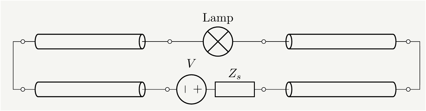
Figure 19: A more accurate representation of Veritasium’s circuit. \(Z_s\) represents the internal resistance of the power source. The switch is not shown for simplicity.
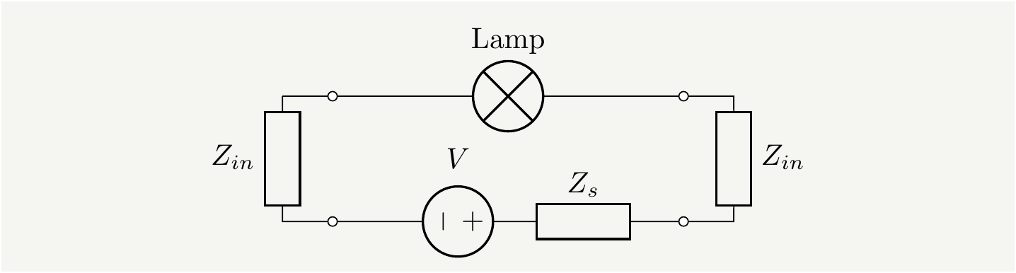
Figure 20: The equivalent circuit where transmission lines are lumped into single circuit elements. We will argue later that this equivalent circuit is missing crucial details.
We can then combine two \(Z_{in}\)’s and call it a day since it becomes (almost) identical to the circuit we looked at earlier in Fig. 11 with the additional source impedance. However, the experimental results look different than the predicted ones[17].

Figure 21: The measured signal in the second video, see the last section. They measure \(Z_0=550\Omega\) for the characteristic impedance and use \(1100\Omega\) for the bulb resistance (\(Z_b\)). They apply \(18V\) to the circuit. The simple model suggests that the bulb voltage should rise to half of the source voltage in the first step and then to the full value. But they see reduced first step (~\(5V\)), and some overshoot beyond the source voltage. Why is that?
The first step of the voltage across the bulb looks smaller than expected whereas the second one overshoots more than the prediction! There is really no way you can tune the values of \(Z\)’s in the formula to explain this. I think what is really going on is a coupling between the wires extending to the left and the ones extending to the right. This is another distributed coupling that sucks energy as the system is powered on. It can be modeled as another transmission line that can be lumped into an impedance which I will refer to as \(Z_c\). I think that we can model the effect of this coupling as an impedance, \(Z_c\), shunting across the bulb and the voltage source (ignoring the cross couplings for simplicity.) The circuit will look like below:
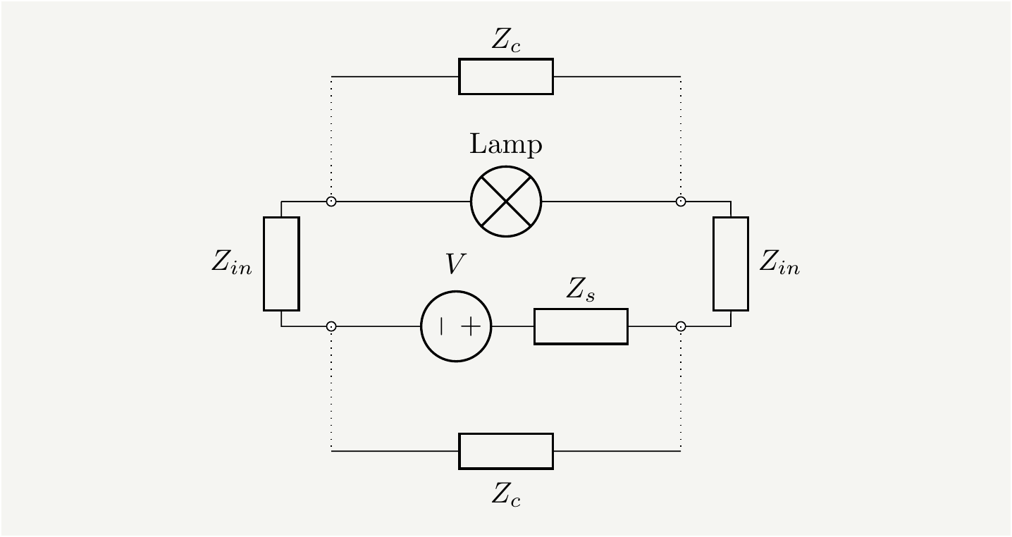
Figure 22: Two shunt impedances are added to model the coupling between the left pair of conductors and the right.
Just concentrating on the new impedance across the bulb, I will argue the following:
At \(t=0\), \(Z_c\) shunts the bulb, reducing the voltage across it. A wave enters into that transmission line, and reflects back from the open end. As the wave comes back and reflects from the bulb (with \(Z_\text{bulb} <Zc\)), it will return the voltage it took away earlier. As this wave comes in, the reflections from the main transmission lines are also arriving simultaneously. So they combine and overshoot the expected peak value. Sometimes it is easier to think about currents rather than voltages. A battery can pull/push current from/to a wire that is connected to nowhere until the wave hits to the end of the wire to find out there is no where to go, and the direction of the current reverses. You can think of this as electron densities being compressed or stretched. This is what is happening here. As the switch is turned on, this cross coupling impedance steals some of the current for a short period of time, and returns it as the waves complete the round trip. This effect should be absent if the experiment is done with one pair of wires, which makes it equivalent to what I considered earlier. We will need more experimental studies to confirm or refute this explanation.
Build your own circuit
This basically visualizes \(v_\text{bulb}(t)=V_b-v(z=0,t)\) from Eq. (92). We take \(Z_0\equiv 100\), in some arbitrary units (you can think it is \(\Omega\)’s)- Notice that we can take ratios of the impedances and make everything unitless. We also take the battery voltage as \(10V\) for simplicity.

Figure 23: Interactive plot that shows the bulb voltage. Battery voltage is taken as \(10V\) and \(Z_0=100\) in some arbitrary units.
Bonus: \(\dot{\mathbf {B}}\) doesn’t induce \(\mathbf {E}\).

Figure 24: Nope, changing magnetic fields do not induce electric fields. Changing electric fields do not induce magnetic fields either.
Although it is not critical to the discussion here, I will also talk a bit about the Maxwell’s equations, particularly the ones that involve \(\mathbf {E}\) and \(\mathbf B\) fields simultaneously, see Eqs. (7) and (8). They are interpreted as “Changing \(\mathbf {E}\) fields create \(\mathbf {B}\) fields and vice-versa.” This interpretation is reinforced in engineering and physics textbooks[18]. It is not semantically correct. You will think that I am now in the crack-pot territory, but first hear me out.
Fields do not induce other fields, it is the sources(charges) that create fields. Since \(\mathbf {E}\) and \(\mathbf {B}\) fields are created from the very same sources, i.e., the electric charges, it may look like they create each other, just like in the case of photon where \(\mathbf {E}\) and \(\mathbf B\) seem to create each other in a perpetual way. No, that is not how it works. \(\mathbf {E}\) and \(\mathbf B\) were created by a charged particle that was accelerated. It emitted oscillatory \(\mathbf {E}\) and \(\mathbf B\) fields, and they are just propagating out- they don’t recreate each other as they go.
To understand this quantitatively, we can re-write Maxwell’s equations is by introducing a scalar \(\phi\) and a vector potential \(\mathbf {A}\), which are created by charges. We can then define fields in terms of these potentials: \[\begin{eqnarray} \mathbf{E}&=&-\mathbf{\nabla}\phi-\frac{\partial \mathbf{A} }{\partial t},\nonumber\\ \mathbf{B}&=&\mathbf{\nabla}\times \mathbf{A}. \tag{93} \end{eqnarray}\] Note that \(\mathbf {E}\) and \(\mathbf {B}\) are now tied to the charges directly, not to each other. They don’t create each other, they are created from the same sources. We can reproduce Faraday’s Law super fast by taking \(\mathbf {\nabla}\times\) of \(\mathbf {E}\): \[\begin{eqnarray} \mathbf {\nabla}\times\mathbf{E}&=&-\mathbf {\nabla}\times\mathbf{\nabla}\phi-\frac{\partial \mathbf {\nabla}\times \mathbf{A} }{\partial t}=-\frac{\partial \mathbf{B} }{\partial t}. \tag{94} \end{eqnarray}\] Deriving Ampere’s law is a bit more involved, but not terribly complicated. It requires some gauge fixing business. The fastest way to get there is to combine \(\phi\) and \(\mathbf {A}\) into a 4-vector: \[\begin{eqnarray} A^{\mu}=(\phi/c,\mathbf{A} ). \tag{95} \end{eqnarray}\] I will not be doing a justice to the topic of gauging by skipping the details, but the redundancy in \(A^{\mu}\) can be removed by requiring \(\partial_\mu A^{\mu}=0\). This results in a neat wave equating for \(A^\mu\): \[\begin{eqnarray} \left( \mu_0\varepsilon_0 \frac{\partial^2}{\partial t^2}-\mathbf{\nabla}^2 \right)A^\mu=\mu_0 j^\mu. \tag{96} \end{eqnarray}\] where \(j^\mu=(c\rho, \mathbf{J})\). With these requirements, take \(\mathbf {\nabla}\times\) of \(\mathbf {B}\) \[\begin{eqnarray} \mathbf {\nabla}\times\mathbf{B}&=&\mathbf {\nabla}\times(\mathbf {\nabla}\times \mathbf{A})=\mathbf {\nabla}\cdot \mathbf {A}-\mathbf {\nabla}^2\mathbf {A}=\mu_0\mathbf{J}+\mu_0\varepsilon_0\frac{\partial\mathbf{E}}{\partial t}. \tag{97} \end{eqnarray}\] As you see, \(\mathbf {\nabla}\times\mathbf{E}\) being equal to \(-\frac{\partial \mathbf{B} }{\partial t}\) or \(\mathbf {\nabla}\times\mathbf{B}\) being equal to \(\mu_0\varepsilon_0\frac{\partial\mathbf{E}}{\partial t}\) does not mean that time varying magnetic fields induce electric fields or vice versa. It is more appropriate to read it as “Certain potential configurations create electric and magnetic fields such that time derivative of the field is equal to the curl of the other field.”
This interpretation is particularly more valid in the case of photon. Rather than defining a photon in terms of perpendicular electric and magnetic fields that travel in phase and claiming that the oscillating fields re-create each other, it is much more intuitive to associate a photon with \(A^\mu\). It automatically creates the perpendicular fields, and behaves as a wave, and although we will not go into that in this post, it naturally arises by gauging a theory. Finally, in quantum mechanics, photon is defined as the quanta of the \(A^\mu\) field.
The bottom line is, electric fields and magnetic fields do not create each other. It is sometimes convenient in conceptual discussions to think that way, but in reality fields are created by their sources, not by time derivative of each other.
The follow up video
Veritasium released a follow up video on April 29, see below. I am glad that in this video he puts most of the emphasis on electric fields rather than the magnetic field or the Poynting’s vector. The Poynting’s vector is mentioned only once in the whole video. This one looks much better!
How Electricity Actually Works, Veritasium
Veritasium is certainly not the first one to create a video on this topic. There is another one from The Science Asylum titled Circuit Energy doesn’t FLOW the way you THINK!. Also note the one from ElectroBOOM titled How Wrong Is VERITASIUM? A bulb and Power Line Story. It is worth to watch that video to see an engineer’s take on the topic.↩︎
I agree with him that thinking about this is as buying electrons is ridiculous. Where would you keep these electrons? I would say it is more like short term renting since you return electrons quickly after you use them. I can even calculate the rent rate. Most of my devices operate at 110V, and my monthly consumption is about \(300\)kwh per month at the rate of \(0.1\) USD per kwh of energy. How many electrons do I rent per hour? It is simply \((300\times 10^3/110)/(1.6\times10^{-19})=1.7\times10^{22}\), which means I am paying \(\$ 6\times10^{-24}\) per electron per hour. ↩︎
We will find out later that it is not an exact replica, but let’s not get ahead of ourselves.↩︎