The Gaussian function

My strongest memory of the class is the very beginning, when he started, not with some deep principle of nature, or some experiment, but with a review of Gaussian integrals. Clearly, there was some calculating to be done.

Due to the central limit theorem, Gaussian functions show up everywhere[2]. One needs to deal with its integrals in various forms. This is an extensive tutorial on Gaussian integrals so that you can evaluate them like a boss! This post is inspired by the masterpiece book “The Principles of Deep Learning Theory” from Robert at al [3], and I took the liberty of borrowing some ideas from their work, including the quoted remarks from Polchinski.

Let us first show how a Gaussian distribution looks like. \[\begin{equation} \mathcal{N}_{\mu,\sigma}(x)=\frac{1}{\sqrt{2 \pi}\sigma}e^{-\frac{\left(x-\mu\right)^2}{2 \sigma^2} }, \tag{1} \end{equation}\] where \(\mu\) is the mean value and \(\sigma\) is the variance.

Assume you are on a beach, and you don’t remember the form of the Gaussian function. What would you do in such a desperate situation? Normal distribution is symmetric around its mean value. So we must have a \((x-\mu)^2\) in the exponent. Note that you can never ever put a parameter which has a dimension in the exponent. You can think of \(x\) as length. \((x-\mu)^2\) has unit \(\text{Length}^2\). Therefore you need to divide \((x-\mu)^2\) by some parameter that has the unit \(\text{Length}^2\), and that is \(2 \sigma^2\). The factor \(2\) is a convention. That fixes the exponent as \(-\frac{\left(x-\mu\right)^2}{2 \sigma^2}\), where you need the negative sign so that the density function is normalizable. How about the prefactor? Remember that normal distribution is a density, and we will soon integrate it over the parameter \(x\). Therefore, it needs to have a unit of \(\text{Length}^{-1}\) so that once you multiply it with \(dx\) you get probability, which is a unitless number. So you need \(1/\sigma\) in front of the exponential. \(\sqrt{2\pi}\) is for normalizing the distribution, which we will derive later. And that is how you can remind yourself the form of the normal distribution.

The pesky error function

Figure 1: Interactive plot showing the normal distribution PDF and CDF.

The central limit theorem

Gaussian function appears everywhere, including statistics, physics, and neural networks [3]. Why is that? It is because of the central limit theorem, which can be loosely defined as follows: If you add up many random variables, their properly normalized sum converges toward a normal distribution irrespective of the type of distribution of the original variables. That is a very strong statement, and justifies the use of normal distribution if you think the end quantity is the sum of many underlying contributors. In the special case of independent and identically distribute random variables \(X_i\) with \(i=1,2,\cdots n\), the central limit theorem can be written as follows: \[\begin{equation} \frac{1}{\sqrt{n}\sigma}\sum_{i=0}^n (X_i-\mu) \sim \mathcal{N}(0,1). \tag{5} \end{equation}\]

The normalization factor

The first integral we will look at is the most basic one. In order to be a proper distribution function, it has to be normalized. Therefore we need to compute the factor that appears in front of the exponential in Eq. (1). We need to evaluate the following integral: \[\begin{equation} I\equiv\int_{-\infty}^{\infty} dx e^{-\frac{\left(x-\mu\right)^2}{2 \sigma^2} }. \tag{6} \end{equation}\] There are many different ways computing the integral in Eq. (6), and I will only discuss the ones I like the most.

Squaring the integral to polarize it

Here is our integral to evaluate: \[\begin{equation} I= \int_{-\infty}^{\infty} dx e^{-\frac{\left(x-\mu\right)^2}{2 \sigma^2} } = \sqrt{2}\sigma \int_{-\infty}^{\infty} dx e^{-x^2}. \tag{7} \end{equation}\] We will do a neat trick and square the integral: \[\begin{equation} I^2= 2\sigma^2 \int_{-\infty}^{\infty} dx e^{-x^2} \int_{-\infty}^{\infty} dy e^{-y^2}= 2\sigma^2 \int_{-\infty}^{\infty} \int_{-\infty}^{\infty} dx dy e^{-(x^2+y^2)}. \tag{8} \end{equation}\] It doesn’t look like we made progress, but we notice that \(dxdy\) is the differential area, and switch to polar coordinates ,as in Fig. 2, to see if that helps.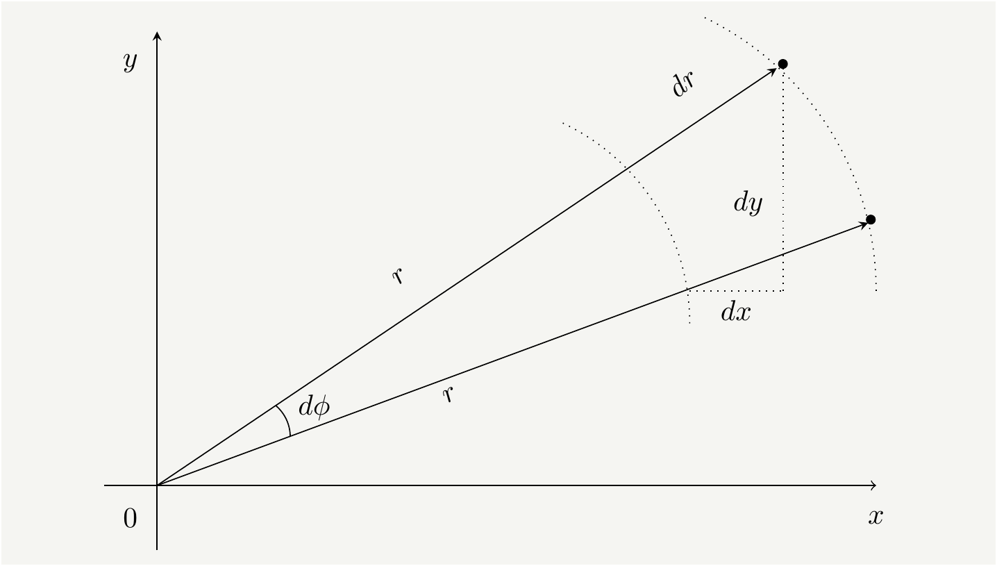

Figure 2: The integral over \(dA\) can be evaluated in Cartesian coordiates with \(dA=dxdy\) or in polar coordinates \(dA=r drd\phi\).

In the polar coordinates we have \(x=r \cos \phi\), \(y=r \sin \phi\), and \(dA= dx dy = r d r d\phi\).

\[\begin{equation} I^2 = \int_{-\infty}^{\infty} \int_{-\infty}^{\infty} d x d y e^{-(x^2+y^2)}=\int_{0}^{\infty} e^{-r^2} r d r \int_{0}^{2\pi} d \phi =\pi\tag{9} \end{equation}\]

Therefore the integral in Eq. (7) has the value \[\begin{equation} I= \int_{-\infty}^{\infty} dx e^{-\frac{\left(x-\mu\right)^2}{2 \sigma^2} } = \sqrt{2\pi}\sigma \tag{10}, \end{equation}\] which is the inverse of the coefficient in the Gaussian distribution in Eq. (1) ensuring that it is properly normalized to \(1\).

Complex contour integral, like a boss!

It is possible to compute the Gaussian integral using complex calculus. As \(e^{-x^2}\) has no zeros itself, we consider a function \(\frac{e^{-x^2}}{g(x)}\), and upgrade the real parameter \(x\) to a complex parameter \(z\), and integrate \(\frac{e^{-z^2}}{g(z)}\) in on a carefully built contour in Fig. 3. The trick is to combine two pieces of complex line integrals to give what we want at the end.

Figure 3: Animated complex contour integration.

The mean, sigma, and all that

\(\mathcal{N}_{\mu,\sigma}(x)\) has a parameter \(\mu\) which is the value around which the distribution is symmetric, see Fig. 1. We can show that the expected value of a random number \(X\sim \mathcal{N}_{\mu,\sigma}\) is \(\mu\) by evaluating the following integral:

\[\begin{eqnarray} \mathbb{E}\left[x\right]&\equiv& \int_{-\infty}^{\infty} dx\, x \mathcal{N}_{\mu,\sigma}(x) =\frac{1}{\sqrt{2\pi}\sigma} \int_{-\infty}^{\infty}dx \,x e^{-\frac{(x-\mu)^2}{2\sigma^2}} =\frac{1}{\sqrt{2\pi}\sigma} \int_{-\infty}^{\infty}dx \,(x-\mu+\mu) e^{-\frac{(x-\mu)^2}{2\sigma^2}} \nonumber\\ &=&\cancelto{0}{\frac{1}{\sqrt{2\pi}\sigma} \int_{-\infty}^{\infty}dx \,(x-\mu) e^{-\frac{(x-\mu)^2}{2\sigma^2}}}+\mu\frac{1}{\sqrt{2\pi}\sigma} \int_{-\infty}^{\infty}dx e^{-\frac{(x-\mu)^2}{2\sigma^2}}=\mu, \tag{11} \end{eqnarray}\] where the first integral vanishes since the integrand is odd.

In order to compute the variance, we have to figure out how to compute the expected value of \((x-\mu)^2\). We can be a bit more generous and compute the expected value of \((x-\mu)^{2n}\) where \(n\) is a positive integer. Note that odd powers of \((x-\mu)\) will have \(0\) as their expected value as they are antisymmetric.

\[\begin{eqnarray} \mathbb{E}\left[(x-\mu)^{2n}\right]&\equiv& \int_{-\infty}^{\infty} dx\, (x-\mu)^{2n} \mathcal{N}_{\mu,\sigma}(x) =\frac{1}{\sqrt{2\pi}\sigma} \int_{-\infty}^{\infty}dx \,(x-\mu)^{2n} e^{-\frac{(x-\mu)^2}{2\sigma^2}}\nonumber\\ &=&\frac{1}{\sqrt{2\pi}\sigma} \int_{-\infty}^{\infty}dx \,(x-\mu)^{2n} e^{-\alpha (x-\mu)^2}\bigg\rvert_{\alpha=\frac{1}{2\sigma^2}} = \frac{1}{\sqrt{2\pi}\sigma}(-1)^n \frac{d^n}{d\alpha^n} \int_{-\infty}^{\infty}dx \,e^{-\alpha (x-\mu)^2}\bigg\rvert_{\alpha=\frac{1}{2\sigma^2}}\nonumber\\ &=&\frac{1}{\sqrt{2\pi}\sigma}(-1)^n \frac{d^n}{d\alpha^n} \sqrt{\pi}\alpha^{-\frac{1}{2}}\bigg\rvert_{\alpha=\frac{1}{2\sigma^2}} =\frac{1}{\sqrt{2}\sigma} \frac{1}{2}\times\frac{3}{2}\times\cdots \times\frac{2n-1}{2} \alpha^{-\frac{2n+1}{2}} \bigg\rvert_{\alpha=\frac{1}{2\sigma^2}}\nonumber\\ &=&1\times 3\times 5\times\cdots \times\frac{2n-1}{2} \sigma^{2 n}=\sigma^{2 n}(2n-1)!! \tag{12}, \end{eqnarray}\] where the double factorial term is defined as \((2n-1)!!\equiv(2n-1)(2n-3)\cdots 1 = \frac{(2n) !}{2^n n!}\).

There is another technique which is known as Feynman’s method. It is similar to what we just did: we differentiated the integrand with respect to the parameter we called \(\alpha\). However, it was kind of an obvious thing to do. Feynman’s method takes this one step further. You insert a parameter by hand and poke that parameter before you set it to the appropriate value(typically \(0\) or \(1\)) at the end. It is an incredibly powerful technique and it is work repeating the calculations to illustrate how it works. Let’s consider the following integral: \[\begin{eqnarray} \mathbb{E}\left[e^{J(x-\mu)}\right]&=&\int_{-\infty}^{\infty} dx\, e^{J(x-\mu)} \mathcal{N}_{\mu,\sigma}(x) =\frac{1}{\sqrt{2\pi}\sigma} \int_{-\infty}^{\infty}dx \, e^{-\frac{(x-\mu)^2}{2\sigma^2}+J(x-\mu)} =\frac{1}{\sqrt{2\pi}\sigma} \int_{-\infty}^{\infty}dx \, e^{-\frac{(x-\mu)^2 -2 \sigma^2 J(x-\mu)}{2\sigma^2}}\nonumber\\ &=&\frac{1}{\sqrt{2\pi}\sigma} \int_{-\infty}^{\infty}dx \, e^{-\frac{\left[x-\mu - \sigma^2 J(x-\mu)\right]^2}{2\sigma^2} +\frac{J^2\sigma^2}{2}}=e^{\frac{J^2\sigma^2}{2}}. \tag{13} \end{eqnarray}\] Note that we can now drop in the term \((x-\mu)^n\) by differentiating the integral with respect to \(J\). \[\begin{eqnarray} \mathbb{E}\left[(x-\mu)^n\right]&=& \left[\left(\frac{d}{dJ}\right)^{2n} \mathbb{E}\left[e^{J(x-\mu)}\right]\right]_{J=0}=\left[\left(\frac{d}{dJ}\right)^{2n} \int_{-\infty}^{\infty} dx\, e^{J(x-\mu)} \mathcal{N}_{\mu,\sigma}(x)\right]_{J=0}\nonumber\\ &=&\frac{1}{\sqrt{2\pi}\sigma} \int_{-\infty}^{\infty}dx \,(x-\mu)^{2n} e^{-\frac{(x-\mu)^2}{2\sigma^2}} =\left[\left(\frac{d}{dJ}\right)^{2n} e^{\frac{J^2\sigma^2}{2}}\right]_{J=0}\nonumber\\ &=&\left[\left(\frac{d}{dJ}\right)^{2n}\left\{ \sum_{i=0}^{\infty}\frac{1}{i!} \left(\frac{\sigma^2}{2}\right)^{i} J^{2i}\right\}\right]_{J=0} = \sigma^{2n}\frac{\left(2n\right) !}{2^n n!}\nonumber\\ &=&\sigma^{2n} (2n-1)!!, \tag{14} \end{eqnarray}\] where the only contribution from the summation comes from \(i=n\) since \(J\) is set to zero after differentiation.

The Matrix representation

There are problems involving Gaussians with multiple variables, and ff the variables are not connected, one can simply separate the integrals to evaluate them individually. For example a Gaussian with two variables will be of the form \(exp\left\{-(x-\mu_x)^2/(2\sigma_x^2)-(y-\mu_y)^2/(2\sigma_y^2)\right\}\) which can be separated as \(exp\left\{-(x-\mu_x)^2/(2\sigma_x^2)\right\}\times exp\left\{-(y-\mu_y)^2/(2\sigma_y^2)\right\}\), and the integrals simply decouple. However, if there are cross terms of the form \(x\,y\), we need to come up with a new set of coordinates to eliminate the cross term. In the jargon of linear algebra, this is referred to as diagonalization. In order to keep the notation simple, let us now upgrade the parameter \(x\) to a vector \(\mathbf{x}=(x_1,x_2,\cdots, x_N)^T\), and consider the following integral: \[\begin{eqnarray} I=\int_{-\infty}^{\infty}d^N\mathbf{x} e^{-\mathbf{x}^T M \mathbf{x}}, \tag{15} \end{eqnarray}\] where \(M\) is an \(N\)-by-\(N\) symmetric positive definite matrix, which is not necessarily a diagonal one. However we can rotate our vector \(\mathbf{x}\) with a rotation matrix \(R\), i.e., \(\mathbf{y}=M\mathbf{x}\) or equivalently \(\mathbf{x}=M^T\mathbf{y}\), such that the rotation operation diagonalizes the matrix \(M\). It works like below: \[\begin{eqnarray} \mathbf{x}^T M \mathbf{x}=\mathbf{y}^T R M R^T \mathbf{y}\equiv \mathbf{y}^T \Lambda \mathbf{y}, \tag{16} \end{eqnarray}\] where \[\begin{equation} \Lambda= R M R^T \tag{17} \end{equation}\] is a diagonal matrix \(\frac{1}{\lambda_i}\delta_{ij}\). Since rotation matrices do not change the volume, the integral measure stays the same. Therefore the integrals decouple in the \(\mathbf{y}\) space:

\[\begin{eqnarray} I&=&\int_{-\infty}^{\infty}d^N\mathbf{x} e^{-\frac{1}{2}\mathbf{x}^T M \mathbf{x}}=\int_{-\infty}^{\infty}d^N\mathbf{y} e^{-\frac{1}{2}\mathbf{y}^T \Lambda \mathbf{y}} =\int_{-\infty}^{\infty}d^N\mathbf{y} e^{-\sum_{i,j}\frac{1}{2\lambda_i}\mathbf{y}_i \delta_{ij} \mathbf{y}_i} =\int_{-\infty}^{\infty}d^N\mathbf{y} e^{-\sum_{i}\frac{y_i^2}{2\lambda_i}}\nonumber\\ &=&\prod_{i} \int_{-\infty}^{\infty}dy_i e^{\frac{y_i^2}{2\lambda_i}} =\prod_{i}\sqrt{2\pi\lambda_i}=\sqrt{\prod_{i}(2\pi\lambda_i)}=\sqrt{|2\pi\Lambda^{-1}|}=\sqrt{|2\pi M^{-1}|}, \tag{18} \end{eqnarray}\] where we used the fact that determinant of a matrix, \(|M|\), is the multiplication of its eigenvalues. Putting the reciprocal of this factor infront gives the normalized Gaussian distribution with multiple variables: \[\begin{eqnarray} \mathcal{N}_{\mathbf{\mu},M}(\mathbf{x})=\frac{1}{\sqrt{|2\pi M^{-1}|}}e^{-\frac{1}{2}(\mathbf{x}-\mathbf{\mu})^T M (\mathbf{x}-\mathbf{\mu})}, \tag{19} \end{eqnarray}\] where we introduced the mean value vector \(\mathbf{\mu}=(\mu_1,\mu_2,\cdots,\mu_N)\).

The Wick contraction

Computation of the moments is very similar to the case of single variable Gaussian. We introduce \(\mathbf{J}\) vector and couple it to \(\mathbf{x}-\mathbf{\mu}\). The exponent becomes: \[\begin{eqnarray} -\frac{1}{2}(\mathbf{x}-\mathbf{\mu})^T M (\mathbf{x}-\mathbf{\mu})+\mathbf{J}^T(\mathbf{x}-\mathbf{\mu}) =-\frac{1}{2}\left(\mathbf{x}-\mathbf{\mu}-(M^{-1})^T\mathbf{J}\right)^T M \left(\mathbf{x}-\mathbf{\mu}-M^{-1}\mathbf{J}\right)+\frac{1}{2}\mathbf{J}^T M^{-1} \mathbf{J}. \tag{20} \end{eqnarray}\] Similar to what we did in Eq. (13), we consider the following integral: \[\begin{eqnarray} \mathbb{E}\left[e^{\mathbf{J}^T(\mathbf{x}-\mathbf{\mu})}\right]&=&\int_{-\infty}^{\infty} d^N\mathbf{x}\, e^{\mathbf{J}(\mathbf{x}-\mathbf{\mu})} \mathcal{N}_{\mathbf{\mu},M}(\mathbf{x}) =\frac{1}{\sqrt{|2\pi M^{-1}|}}\int_{-\infty}^{\infty} d^N\mathbf{x}\, e^{\mathbf{J}(\mathbf{x}-\mathbf{\mu})} \mathcal{N}_{\mathbf{\mu},M}(\mathbf{x})\nonumber\\ &=&\frac{1}{\sqrt{|2\pi M^{-1}|}}\int_{-\infty}^{\infty} d^N\mathbf{x}\, e^{-\frac{1}{2}\left(\mathbf{x}-\mathbf{\mu}-(M^{-1})^T\mathbf{J}\right)^T M \left(\mathbf{x}-\mathbf{\mu}-M^{-1}\mathbf{J}\right)+\frac{1}{2}\mathbf{J}^T M^{-1} \mathbf{J}}\nonumber\\ &=&e^{\frac{1}{2}\mathbf{J}^T M^{-1} \mathbf{J}}=e^{\frac{1}{2}\sum_{k,l}J_k M^{-1}_{kl}J_l }. \tag{21} \end{eqnarray}\] Let us first shift the variables by their mean values to simplify the notation a bit: \(\mathbf{z}=\mathbf{x}-\mathbf{\mu}\). In the \(\mathbf{z}\) coordinates, we can compute the moments easily as follows: \[\begin{eqnarray} \mathbb{E}\left[z_{i_1}z_{i_2}\cdots z_{i_{2n}}\right]&=& \left[\frac{d}{dJ_{i_1}}\frac{d}{dJ_{i_2}}\cdots \frac{d}{dJ_{i_{2n}}} \mathbb{E}\left[e^{\mathbf{J}\mathbf{z}}\right]\right]_{\mathbf{J}=0} =\left[\frac{d}{dJ_{i_1}}\frac{d}{dJ_{i_2}}\cdots \frac{d}{dJ_{i_{2n}}} \int_{-\infty}^{\infty} d^N\mathbf{z}\, e^{\mathbf{J}\mathbf{z}} \mathcal{N}_{\mathbf{0},M}\right]_{\mathbf{J}=0}\nonumber\\ &=&\left[\frac{d}{dJ_{i_1}}\frac{d}{dJ_{i_2}}\cdots \frac{d}{dJ_{i_{2n}}} e^{\frac{1}{2}\mathbf{J}^T M^{-1} \mathbf{J}} \right]_{\mathbf{J}=0}=\left[\frac{d}{dJ_{i_1}}\frac{d}{dJ_{i_2}}\cdots \frac{d}{dJ_{i_{2n}}}\left\{ \sum_{i=0}^{\infty}\frac{1}{i!} \left(\frac{1}{2}\sum_{k,l}J_k M^{-1}_{kl}J_l\right)^{ i} \right\}\right]_{J=0}\nonumber\\ &=&\frac{1}{2^n n!}\frac{d}{dJ_{i_1}}\frac{d}{dJ_{i_2}}\cdots \frac{d}{dJ_{i_{2n}}}\left(\sum_{k,l}J_k M^{-1}_{kl}J_l\right)^n. \tag{22} \end{eqnarray}\] Note that the derivative operator will isolate the corresponding indices of the matrix \(M^{-1}.\) For example: \[\begin{eqnarray} \mathbb{E}\left[z_{i_1}z_{i_2}\right]&=&\frac{1}{2} \frac{d}{dJ_{i_1}}\frac{d}{dJ_{i_2}}\sum_{k,l}J_k M^{-1}_{kl}J_l= M^{-1}_{i_{1}i_{2}}, \tag{23} \end{eqnarray}\] where we got a factor of \(2\) from the differentiation which canceled the prefactor. In fact, this cancellation will hold for any \(n\). Therefore we can write the expectation value as summation of all pairs coupled with the matrix \(M^{-1}\):

\[\begin{eqnarray} \mathbb{E}\left[z_{i_1}z_{i_2}\cdots z_{i_{2n}}\right]=\sum_{\text{pairs}}M^{-1}_{p^1_1 p^1_2}M^{-1}_{p^2_1 p^2_2}\cdots M^{-1}_{p^n_1 p^n_2} \,\tag{24} \end{eqnarray}\] where \(p^k_1\) and \(p^k_2\) for a given \(k\) represent two indices paired together, and the sum is over all such possible pairs. For example, for \(n=2\) we get: \[\begin{eqnarray} \mathbb{E}\left[z_{i_1}z_{i_2}z_{i_3}z_{i_4}\right]=\sum_{\text{pairs}}M^{-1}_{p^1_1 p^1_2}M^{-1}_{p^2_1 p^2_2}= M^{-1}_{i_{1}i_{2}} M^{-1}_{i_{3}i_{4}}+M^{-1}_{i_{1}i_{3}} M^{-1}_{i_{2}i_{4}}+M^{-1}_{i_{1}i_{4}} M^{-1}_{i_{2}i_{3}}. \tag{25} \end{eqnarray}\]

The formula in (24) is the Wick’s theorem and it appears frequently in quantum field theory.