![Left: an image of L4C geophone, right: cartoon of inner mechanics. Credit: [@Bowden03calibrationof]](L4C.png)
Figure 1: Left: an image of L4C geophone, right: cartoon of inner mechanics. Credit: [1]
| name | age | gender |
|---|
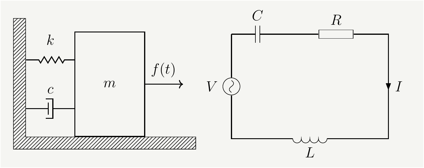
Figure 2: Left:Mass-Spring system with damping driven by an external force, Right: RLC circuit driven by an external voltage source
| Parameter | Description | Parameter | Description |
|---|---|---|---|
| \(k\) | Spring constant | \(C\) | Capacity |
| \(c\) | Damping coefficient | \(R\) | Resistance |
| \(m\) | mass of the object | \(L\) | inductance |
| \(f(t)\) | External force | \(V(t)\) | External Voltage |
Although they are totally different physical systems, the differential equations governing them are very similar, and they can be written as:
\[\begin{eqnarray} m \frac{d^2x}{dt^2}+c \frac{dx}{dt}+k x&=&f(t)\quad \text{(Newton's second law)} \tag{1}\\ L \frac{d^2Q}{dt^2}+R \frac{dQ}{dt}+\frac{ Q}{C}&=&V(t)\quad \text{(Kirchhoff's Voltage Law)}\tag{2}.\\ \end{eqnarray}\]
The parameters are described in Table 2.
Analytical model
Let’s concentrate on Eq. (1) , and divide the equation by \(m\). The simplified differential equation for forced harmonic oscillator with damping reads: \[\begin{eqnarray} \ddot{x}+ 2\zeta \omega_0 \dot{x}+ \omega_0^2 x&=& \frac{ f(t)}{m} ,\, x(0)=x_0, \,\text{and}\,\dot{x}(0)=\dot{x}_0,\tag{3} \end{eqnarray}\] where \(\dot x\equiv\frac{dx}{dt}\), \(\omega_0\equiv\sqrt{\frac{k}{m}}\) is the natural frequency of the oscillation, and \(\zeta\equiv\frac{c}{2\sqrt{mk}}\) is the damping ratio. We also included the initial conditions.
We are dealing with an in-homogeneous linear differential equation with constant coefficients. One of the best tools to solve such equations is the Laplace transformation:
\[\begin{eqnarray} X(s)=\mathcal{L}\big[x(t)\big]=\int_0^\infty dt \, e^{-s \,t} x(t) \tag{4}. \end{eqnarray}\]
The nice feature of the Laplace transformation is that it converts differential equations to algebraic equations. It follows from the transformation property of the derivatives:
\[\begin{eqnarray} \mathcal{L}\big[\dot{x}(t)\big]&=&\int_0^\infty dt \, e^{-s \,t} \frac{dx}{dt}=\int_0^\infty dt \,\frac{d}{dt}\big(e^{-s \,t} x\big)-\int_0^\infty dt \big(\frac{d}{dt}e^{-s \,t}\big) x\\\nonumber &=& \big(e^{-s \,t} x\big)\bigg\rvert_0^\infty+s\int_0^\infty dt e^{-s \,t} x= s X(s)- x_0 \tag{5}. \end{eqnarray}\]
Similarly the second order derivative transforms as \[\begin{eqnarray} \mathcal{L}\big[\ddot{x}(t)\big]&=& s \mathcal{L}\big[\dot{x}(t)\big]- \dot{x}_0 =s^2 X(s) -s x_0 -\dot{x}_0 \tag{6}. \end{eqnarray}\]
Laplace transforming Eq. (3) we get \[\begin{eqnarray} s^2 X -s x_0 -\dot{x}_0+ 2\zeta \omega_0(s X- x_0)+\omega_0^2 X=\frac{ 1}{m} F(s) \tag{7}. \end{eqnarray}\] Solving Eq. (7) for \(X\), we get
\[\begin{eqnarray} X&=&\frac{s x_0+ 2\zeta \omega_0x_0+\dot{x}_0}{s^2 +2 \zeta \omega_0 s+\omega_0^2 }+\frac{1}{m}\frac{F(s)}{s^2 +2 \zeta \omega_0 s+\omega_0^2 }\nonumber\\ &=&\frac{(s+ \zeta \omega_0)x_0+ \zeta \omega_0 x_0+\dot{x}_0}{(s + \zeta \omega_0)^2 +\omega_0^2(1 -\zeta^2)}+\frac{1}{m}\frac{F(s)}{(s + \zeta \omega_0)^2 +\omega_0^2(1 -\zeta^2)} \tag{8}. \end{eqnarray}\] The first term in Eq. (8) is related to the initial conditions, and the excitations associated with this term will die out due to damping. The second term relates the response of the system to the external force. The transfer function of the system is given by \[\begin{eqnarray} H(s)=\frac{X(s)}{F(s)}\bigg\rvert_{x_0=0=\dot{x}_0}&=&\frac{1}{m}\frac{1}{(s + \zeta \omega_0)^2 +\omega_0^2(1 -\zeta^2)} \tag{9}. \end{eqnarray}\]
Response to a sinusoidal force
Although we will concentrate mostly on the transfer function, it is possible to evaluate the inverse Laplace transform if the functional form of the driving force is known. It is a good exercise to calculate the time domain functions when the system is driven by a sinusoidal force. Let’s assume that \(f(t)\) is of the following form:
\[\begin{eqnarray} f(t)&=&f_0\sin(\omega t). \tag{10} \end{eqnarray}\] Its Laplace transform is given by: \[\begin{eqnarray} F(s)\equiv \mathcal{L}\big[f(t)\big]=\frac{f_0 \omega}{s^2+\omega^2}. \tag{11} \end{eqnarray}\] We will have to do some partial fraction expansion: \[\begin{eqnarray} \frac{1}{\left((s + \zeta \omega_0)^2 +\omega_0^2(1 -\zeta^2)\right)(s^2+\omega^2)}=\frac{A(s+\zeta \omega_0)+B}{(s + \zeta \omega_0)^2 +\omega_0^2(1 -\zeta^2)}+\frac{Cs+D}{s^2+\omega^2}, \tag{12} \end{eqnarray}\] which will be easy to convert back to time domain since they will correspond to sines and cosines with exponential functions in front. We now need to figure out \(A\), \(B\), \(C\) and \(D\). If we were to equate the denominators and sum up the resulting numerators, we will see that, in order to set the coefficient of the \(s^3\) term in the numerator to zero we will need \(A=-C.\) To relate \(C\) and \(D\) we can multiply (12) by \(s-i\omega\) and then set \(s=i\omega.\) This will remove the first term on the right hand side and yield:
\[\begin{eqnarray} i\omega C+D=\frac{1}{(i\omega + \zeta \omega_0)^2 +\omega_0^2(1 -\zeta^2)}. \tag{13} \end{eqnarray}\] This is a complex equation, and splitting it into the real and imaginary part, we get: \[\begin{eqnarray} D(\omega_0^2-\omega^2)-2C \omega^2 \omega_0\zeta&=&1,\nonumber\\ C\omega(\omega_0^2-\omega^2)+2D \omega \omega_0\zeta&=&0. \tag{14} \end{eqnarray}\] Inverting it results in: \[\begin{eqnarray} C&=&\frac{-2 \omega_0\zeta}{(\omega_0^2-\omega^2)^2+4\omega^2\omega_0^2\zeta^2},\nonumber\\ D&=&\frac{\omega_0^2-\omega^2}{(\omega_0^2-\omega^2)^2+4\omega^2\omega_0^2\zeta^2}. \tag{15} \end{eqnarray}\] Finally, setting \(s=-\zeta \omega_0\), and going trough some algebra we get. \[\begin{eqnarray} B&=&\frac{\omega^2 -\omega_0^2+2\omega_0^2\zeta^2}{(\omega_0^2-\omega^2)^2+4\omega^2\omega_0^2\zeta^2}. \tag{16} \end{eqnarray}\]
We can now inverse transform Eq. (8) using elementary properties of the transformation:
\[\begin{eqnarray} x(t)&=&\mathcal{L}^{-1}\big[X(s)\big]. \tag{17} \end{eqnarray}\]
Inverse Laplace transformation yields: \[\begin{eqnarray} x(t)&=&\left[x_0 \cos(\omega_0\sqrt{1 -\zeta^2} \,t)+\frac{ \zeta \omega_0 x_0+\dot{x}_0}{\omega_0\sqrt{1 -\zeta^2}}\sin(\omega_0\sqrt{1 -\zeta^2} \,t)\right]e^{-\zeta \omega_0 t}\nonumber\\ &&+\frac{2f_0 \omega}{m}\frac{ \omega_0\zeta}{(\omega_0^2-\omega^2)^2+4\omega^2\omega_0^2\zeta^2}e^{-\zeta \omega_0 t}\cos(\omega_0\sqrt{1 -\zeta^2} \,t)\nonumber\\ &&+\frac{f_0 \omega}{m}\frac{1}{\omega_0\sqrt{1 -\zeta^2}}\frac{\omega^2 -\omega_0^2+2\omega_0^2\zeta^2}{(\omega_0^2-\omega^2)^2+4\omega^2\omega_0^2\zeta^2}e^{-\zeta \omega_0 t}\sin(\omega_0\sqrt{1 -\zeta^2} \,t)\nonumber\\ &&-\frac{2f_0 \omega}{m}\frac{ \omega_0\zeta}{(\omega_0^2-\omega^2)^2+4\omega^2\omega_0^2\zeta^2}\cos(\omega \,t)+\frac{f_0 }{m}\frac{\omega^2 -\omega_0^2}{(\omega_0^2-\omega^2)^2+4\omega^2\omega_0^2\zeta^2}\sin(\omega \,t). \tag{18} \end{eqnarray}\] We can do one last touch and combine the last two terms into as single function with a phase shift. The full solution with damping, and with \(f(t)=f_0\sin(\omega\, t),\quad\) can be written as: \[\begin{eqnarray} x(t)&=&\left[x_0 \cos(\omega_0\sqrt{1 -\zeta^2} \,t)+\frac{ \zeta \omega_0 x_0+\dot{x}_0}{\omega_0\sqrt{1 -\zeta^2}}\sin(\omega_0\sqrt{1 -\zeta^2} \,t)\right]e^{-\zeta \omega_0 t}\nonumber\\ &+&\frac{f_0 \omega e^{-\zeta \omega_0 t}}{m[(\omega_0^2-\omega^2)^2+4\omega^2\omega_0^2\zeta^2]}\left[2\omega_0\zeta\cos(\omega_0\sqrt{1 -\zeta^2} \,t)+\frac{\omega^2 -\omega_0^2+2\omega_0^2\zeta^2}{\omega_0\sqrt{1 -\zeta^2}}\sin(\omega_0\sqrt{1 -\zeta^2} \,t)\right]\nonumber\\ &+&\frac{ f_0}{m\sqrt{(\omega_0^2-\omega^2)^2+4\omega^2\omega_0^2\zeta^2}}\sin(\omega \,t-\delta), \tag{19} \end{eqnarray}\] where \(\delta\equiv \arctan\left[\frac{2\omega\,\omega_0\zeta}{\omega_0^2-\omega^2}\right]\,\,\), the first line is related to the initial conditions, the second and third lines are the transient response, and finally the last line is the steady state solution.- At later times, \(t\gg1/(\zeta \omega_0)\), i.e., in the steady state, only the last term survives.
- The \(x(t)\) is sinusoidal, but it will lag by a phase \(\delta\).
- The system will enter in resonance at \(\omega=\omega_0\sqrt{1-2\zeta}\).
- The value of the resonance amplitude is \(f_0/(2\omega_0^2\zeta\sqrt{1-\zeta^2})\).
- At \(\zeta=0\) (no damping), the amplitude diverges. We need to go back and study this case carefully.
Resonances at zero damping: The final solution runs into problems when we consider \(\zeta=0\) and \(\omega=\omega_0\): the coefficient of the steady state solution diverges. This is because of the assumptions we made when we were inverting \(X(s)\). At \(\zeta=0\) and \(\omega=\omega_0\), two poles will merge and create a second order pole. Let’s take a closer look:
\[\begin{eqnarray} \lim_{\zeta\rightarrow 0,\,\omega\rightarrow\omega_0}\frac{1}{\left((s + \zeta \omega_0)^2 +\omega_0^2(1 -\zeta^2)\right)(s^2+\omega_0^2)}=\frac{1}{(s^2+\omega_0^2)^2}. \tag{20} \end{eqnarray}\] We can figure out how to inverse transform it by exploiting few features of the Laplace transforms as follows:
\[\begin{eqnarray} \mathcal{L}^{-1}\left[\frac{1}{(s^2+\omega_0^2)^2}\right]&=&\mathcal{L}^{-1}\left[-\frac{1}{2s}\frac{d}{ds}\left(\frac{1}{s^2+\omega_0^2}\right)\right]=-\frac{1}{2}\int_0^td\tau \tau \frac{\sin (\omega_0\tau)}{\omega_0}\nonumber\\ &=&-\frac{1}{2 \omega_0}\frac{d}{d\omega_0}\int_0^td\tau \cos (\omega_0\tau)=-\frac{1}{\omega_0}\frac{d}{d\omega_0}\left[\frac{\sin(\omega_0 t)}{\omega_0}\right]=\frac{\sin(\omega_0 t)-\omega_0 t\cos(\omega_0 t)}{2\omega_0^3}. \tag{21} \end{eqnarray}\]
The full solution at the resonance frequency (\(\omega=\omega_0\,\) ) with no damping (\(\zeta=0\)) is:
\[\begin{eqnarray} x(t)&=&\left[x_0 \cos(\omega_0\,t)+\frac{\dot{x}_0}{\omega_0}\sin(\omega_0 \,t)\right]+\left[\frac{f_0}{2 m\omega_0^2}\left( \sin(\omega_0 t)-\omega_0 t\cos(\omega_0 t)\right)\right].\tag{22} \end{eqnarray}\] This shows that the amplitude will grow with time. In reality the model will break at some point since the amplitude of oscillations cannot grow indefinitely. (For example, the spring will literally break if it is stretched too far.)
Visuals
The fact that we can’t change the parameters of the seismometer at will should not stop us from having some fun with fiddling around with seismometer parameters to observe the resulting motion and signal. The interactive plot in Fig. 3 shows the position of the mass, as described in Eq. (19), and the speed of the motion. The seismometer signal is proportional to the speed of the test mass, see Eq. (24).

Figure 3: The position and veleocity of a damped and forced harmonic oscillator. The right axis shows the speed of the mass, which is also proportional to the measured voltage.
Impedance vs frequency
Note that we are trying to isolate the impedance associated with the dynamics. The seismometer has its intrinsic resistance(\(R\)) and inductance(\(L\)) which we will simply add on as \(L s + R\). We can easily convert the relation between \(x\) and \(i\) in Eq. (23) into a relation between \(v_g\) and \(i\) by taking another derivative: \[\begin{eqnarray} \frac{d^2}{dt^2}{\dot{x}}+ 2\zeta \omega_0 \frac{d}{dt}\dot{x}+ \omega_0^2 \dot x&=& \frac{ B l \dot i}{m}.\tag{25} \end{eqnarray}\] Replacing \(\dot{x}\) with \(\frac{v_g}{Bl}\) yields
\[\begin{eqnarray} \ddot v_g+ 2\zeta \omega_0 \dot v_g+ \omega_0^2 v_g&=& \frac{ B^2 l^2 \dot i}{m}.\tag{26} \end{eqnarray}\]
In the \(s\) space, the relation between the current and the voltage is given by: \[\begin{eqnarray} V_g(s)=\frac{ B^2 l^2}{m} \frac{s}{s^2+2\zeta \omega_0 s +\omega_0^2}I(s)\equiv Z(s) I(s)\tag{27}, \end{eqnarray}\] where we identify the factor in front of \(I(s)\) as the impedance associated with the dynamics of the mass. Finally, we can add the intrinsic impedance of the coil to get the complete impedance as \[\begin{eqnarray} Z(s)=L s + R+ G^2 \frac{s}{s^2+2\zeta \omega_0 s +\omega_0^2}=\frac{L s^3 + (2 L\zeta \omega_0+R) s^2+ (2 \zeta \omega_0 R+\omega_0^2 L+G^2)s+R \omega_0^2 }{s^2+2\zeta \omega_0 s +\omega_0^2} \tag{28}, \end{eqnarray}\] where we defined \(G^2=\frac{ B^2 l^2}{m}\).
Table 3 shows the values of the device parameters.| Parameter | Description | Value |
|---|---|---|
| \(m\) | mass | \(1\)[kg] |
| \(R\) | Resistance | \(5500[\Omega]\) |
| \(L\) | Inductance | \(6050\)[mH] |
| \(G\) | Coupling | \(276[\frac{V}{m/s}]\) |
| \(\zeta\) | Damping | 0.28 |
We can plot the impedance as a function of frequency by plugging in \(s=j 2\pi f\) and the numerical values from Table 3 into Eq. (28), we can compute the impedance as follows:
\[\begin{eqnarray} Z(f)&=& \frac{6.05 s^3 + 5521 s^2+ 95976 s+217131 }{s^2+ 3.52 s +39.48}\bigg\rvert_{s=j 2\pi f} \tag{29}. \end{eqnarray}\]
Figure 4 shows the impedance of the device.
Figure 4: Impedance as a function of the frequency. Right axis shows the angle of the impedance.