Introduction
In optimization problems with constraints, one tries to find the extrema of a function while satisfying the contraints imposed. Consider a function, \(f(x,y)\), and assume we want to find the location \((x_0,y_0)\) for which \(f(x_0,y_0)\) assumes its maximum, and at the same time we want a constrain function to be satisfies: \(g(x_0,y_0)=0\). One can solve this problem using brute force:
- Require \(\mathbf{\nabla} f(x,y)\vert_{(x_0,y_0)}=0\) and \(g(x_0,y_0)=0\).
- Solve these two equations with two unknowns.
Although it is technically possible to solve it this way, it may require us to invert complicated functions which might be hard to do. It gets even harder as we introduce more variables and constraints. We can do better than that!
Let us consider a contour curve of \(f\), which is the pairs of numbers \((x,y)\) for which \(f(x,y)=k\). We want \(k\) to be as large as possible while satisfying \(g(x_0,y_0)=0\). To illustrate the method, let us take the following functions:
\[\begin{eqnarray} f(x,y)=y^2-x^2, \quad g(x,y)=x^2+y^2-1, \tag{1} \end{eqnarray}\] which are shown in Fig. 1.
Figure 1: Showing the \(x,y\) values satisfying \(f(x,y)=k\), and the constraint function \(g(x,y)=x^2+y^2-1=0\), which is the unit circle. You can change the value of \(k\) and observe how the curve moves. Also follow the slopes of the curves at one of the intersection points.
If there was no constraint, we would increase the value of \(k\) indefinitely. However, we are required to find a solution \((x_0,y_0)\) that satisfies \(g(x_0,y_0)=0\), which means two curves have to pass through the point \((x_0,y_0)\). As you tune the value of \(k\), you realize that you can make the curves to intersect at different points. The optimal solution is the one at which two curves touch each other, and, for this particular example, we can graphically see that it happens at \(k=1\) and \((x_0,y_0)=(0,1)\).
How do we solve this analytically though? Note that in this critical point, two curves are barely touching each other. More precisely, they are tangent to each other at that point, i.e., they have the same value and the same slope. Since the tangents are the same, the vector which is perpendicular to the tangents must be the same too. And that perpendicular vector is nothing but the gradient. Note that we are limiting ourselves to a two-dimensional problem for pedagogical reasons. The observation above holds for any dimension. Let’s prove that gradient vector is indeed perpendicular to the curve. In a generic case, \(f\) can be a function of multiple variables: \(f=f(x_1,x_2,\cdots,x_n)\) where \(\mathbf{x}=(x_1,x_2,\cdots,x_n)\) is an \(n\) dimensional vector. The level surface of this function is composed of \(\mathbf{x}\) values such that \(f(\mathbf{x}_0)=k\), which defines an \(n-1\) dimensional level surface. What we want to prove is that for any point on the level surface, \(f(\mathbf{x}_0)=k\), the gradient of \(f\), i.e., \(\mathbf{\nabla}f\vert_{\mathbf{x}_0}\) is perpendicular to the surface.
Let us take an arbitrary curve on this surface, \(\mathbf{x}(t)\), parameterized by a parameter \(t\), and assume it passes through \(\mathbf{x}_0\) at \(t=t_0\). On the surface \(f(\mathbf{x}(t))=f\left(x_1(t),x_2(t),\cdots,x_n(t)\right)= k\). Let’s take the parametric derivative of \(f\) and apply the chain rule.
\[\begin{eqnarray} \frac{df}{dt}=0=\sum_{i=1}^n \left.\frac{\partial f}{\partial x_i}\right\vert_{\mathbf{x}_0}\left. \frac{d x_i}{dt}\right\vert_{t_0} = \left.\mathbf{\nabla} f\right\vert_{\mathbf{x}_0} \cdot \dot{\mathbf{x}}\vert_{t_0} \tag{2}, \end{eqnarray}\] where we defined \(\dot{\mathbf{x}}\vert_{t_0}=\left.\frac{d\mathbf{x}(t)}{dt}\right\vert_{t_0}\), which is nothing but the tangent line. Therefore we conclude that the gradient is perpendicular to the tangent lines on the surface.
This exercise tells us that the gradients of the function we want to optimize is parallel to the gradient of the constraint function. That is:
\[\begin{eqnarray} \left.\mathbf{\nabla} f \right\vert_{\mathbf{x}_0}= \lambda \left.\mathbf{\nabla} g\right\vert_{\mathbf{x}_0}\tag{3}, \end{eqnarray}\] where the constant \(\lambda\) is the Lagrange multiplier. And keep in mind that we also need to satisfy \(g(\mathbf{x}_0)=0\) We can neatly combine these to requirements by defining a new function:
\[\begin{eqnarray} h(\mathbf{x},\lambda)= f(\mathbf{x}) -\lambda g(\mathbf{x})\tag{4}, \end{eqnarray}\] which can be optimized by requiring
\[\begin{eqnarray} \left.\mathbf{\nabla} h\right\vert_{\mathbf{x}_0}=0, \quad \text{and}\quad \left.\frac{\partial h}{\partial \lambda}\right\vert_{\mathbf{x}_0}=0 \tag{5}. \end{eqnarray}\] The bottom line is that the constraint itself is mixed into the function that we want to optimize. The expression in (5) has equal number of equations and unknowns, so we can solve for \(\mathbf{x}_0\) and \(\lambda\).
Examples
Let us consider a few examples to illustrate the use of Lagrange multiplier.
The problem in the intro
We want to solve the problem we looked at earlier in Eq. (1) using the technique we learned. The combined function to optimize is: \[\begin{eqnarray} h(\mathbf{x},\lambda)= f(\mathbf{x}) -\lambda g(\mathbf{x})= y^2-x^2-\lambda(x^2+y^2-1)=y^2(1-\lambda)-x^2(1+\lambda)-\lambda \tag{6}. \end{eqnarray}\] In order to optimize \(h\), we require the following:
\[\begin{eqnarray} \left.\mathbf{\nabla} h\right\vert_{\mathbf{x}_0}&=&0= \left(2y_0(1-\lambda),-2x_0(1+\lambda) \right),\nonumber\\ \left.\frac{\partial h}{\partial \lambda}\right\vert_{\mathbf{x}_0}&=&0=x_0^2+y_0^2-1 \tag{7}. \end{eqnarray}\] We have two options:
- \(y_0=0\, \&\lambda=-1\) satisfies the first line. Additionally, we need \(x_0=1\) to satisfy the second line.
- This gives \(f(x_0,y_0)=-1\), which is the minimum value of the function \(f\) with the constraint \(g\).
- \(x_0=0\, \&\lambda=1\) also satisfies the first line. Additionally, we need \(y_0=1\) to satisfy the second line.
- This gives \(f(x_0,y_0)=1\), which is the maximum value of the function \(f\) with the constraint \(g\).
Shannon entropy
Shannon entropy[1] for a continuous probability distribution \(p(x)\) is expressed as follows see: \[\begin{eqnarray} S=-\int dx p(x) \log\left(p(x)\right), \tag{8} \end{eqnarray}\] where the integral is evaluated over the space \(p(x)\) is defined. What kind of distribution would maximize the entropy? One can anticipate that it has to be the uniform distribution defined in a specific range. And we can easily prove that using calculus of variations with Lagrange multipliers. The Lagrange multiplier comes in to satisfy the normalization of the probability density: \[\begin{eqnarray} \int dx p(x) =1. \tag{9} \end{eqnarray}\] Combining the condition with the target function to maximize, Eq. (8), we have the following integral to maximize: \[\begin{eqnarray} I=-\int dx p(x) \log\left(p(x)\right)-\lambda\left( \int dx p(x)-1 \right)=- \int dx p(x) \left( \log\left(p(x)\right) +\lambda \right)+\lambda \tag{10} \end{eqnarray}\]
Now move the function \(p(x)\) to \(p(x)+\delta(x)\), and require that \(\delta I=0\) for the \(p(x)\) that maximizes \(I\). This yields: \[\begin{eqnarray} \delta I=-\int dx \delta p(x) \left[ \log\left(p(x)\right)+1 +\lambda \right]=0. \tag{11} \end{eqnarray}\] Since \(\delta p(x)\) is totally arbitrary, we need \(\log\left(p(x)\right)+1 +\lambda=0\). Furthermore, as \(\lambda\) is just a constant, this shows that \(p(x)\) is also a constant. Let’s assume that we are interested in distributions defined in the range \([a,b]\). The normalization condition in Eq. (9) uniquely defines the value of the constant as \(\frac{1}{b-a}\).
Boltzman distribution
Consider a system with \(m\) states. An occupation number is the number of systems, \(n\), occupying a given \(i^\text{th}\) state, and we will denote this number as \(n_i\). Given \(m\) such states, i.e., \(i\in\{1,2,\cdots,m\}\), we are interested in finding the total number of possible ways to redistribute the systems among the states. This is illustrated in Fig. 2.
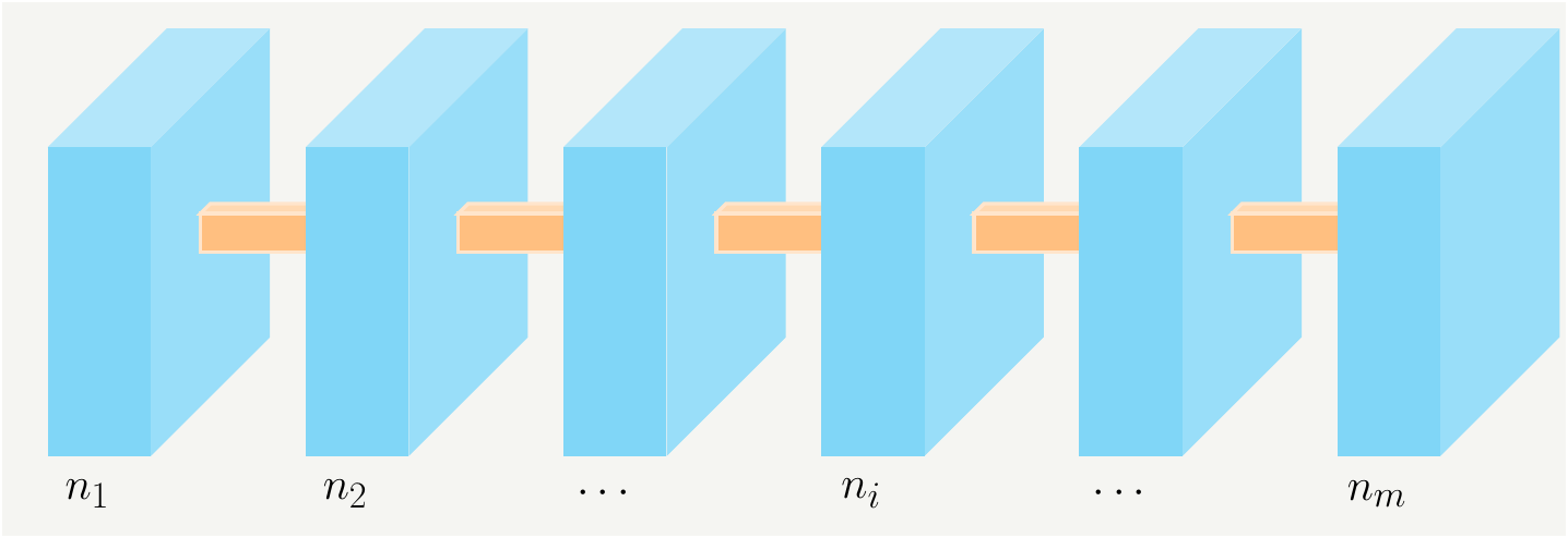
Figure 2: \(m\) boxes with given occupation numbers \(n_i\).
We assume that the total number of occupation number is fixed, we will define it as \(N\): \[\begin{eqnarray} N\equiv\sum_{i=1}^m n_i. \tag{12} \end{eqnarray}\] For a randomly selected system, the probability of that system to be in state \(i\) is the ratio of the number of states in the \(i^\text{th}\) and the total number of states: \[\begin{eqnarray} p_i= \frac{n_i}{N}, \tag{13} \end{eqnarray}\] which results in a normalized probability distribution: \[\begin{eqnarray} \sum_{i=1}^m p_i= 1. \tag{14} \end{eqnarray}\] We also need to make sure that total energy is conserved: \[\begin{eqnarray} \sum_{i=1}^m E_i n_i =N \sum_{i=1}^m E_i \frac{n_i}{N} =N\sum_{i=1}^m E_i p_i=N E, \tag{15} \end{eqnarray}\] where \(E\) is the average energy. While keeping the occupation numbers fixed, we can shuffle systems around to create different configurations. For \(N\) systems, we get \(N!\) shufflings. However, we should remove the overcounting within the states with \(n_i\) as the occupation number. Therefore the total number of combination to create such as system is: \[\begin{eqnarray} C= \frac{N!}{\prod_{i=1}^{m} n_i!}. \tag{16} \end{eqnarray}\] We can now take the log of \(C\) and use the Stirling approximation: \(n!=\sqrt{2\pi n}\left(\frac{n}{e}\right)^n\): \[\begin{eqnarray} log(C)&=& log(N!)-\sum_{i=1}^mlog(n_i!)=N log(N)-N-\sum_{i=1}^mnilog(n_i)+\sum_{i=1}^mn_i+\mathcal{O}(1)\nonumber\\ &=&-N \sum_{i=1}^m\frac{ni}{N}log\left(\frac{ni}{N}\right)=-N\sum_{i=1}^m p_i log(p_i). \tag{17} \end{eqnarray}\] We have shown earlier that this expression is maximized when \(p_i\) are equally likely, which was the case for the Shannon entropy. However, it is very different for this case since we have an additional constraint now, as described in Eqs. (12) and (14). We will multiply these constraints with Lagrange multipliers which we will call \(\alpha\) and \(\beta\), and subtract them from the original function in Eq. (17). Therefore the combined function becomes: \[\begin{eqnarray} h(p_i,\alpha,\beta) &=& -N \sum_{i=1}^m p_i log(p_i)- \alpha\left(\sum_{i=1}^m n_i-N \right) - \beta\left(N \sum_{i=1}^m E_i p_i -N E \right)\nonumber\\ &=&-N\left\{ \sum_{i=1}^m p_i log(p_i)- \alpha\left(\sum_{i=1}^m p_i-1 \right) - \beta\left( \sum_{i=1}^m E_i p_i - E \right) \right\} \tag{18} \end{eqnarray}\] Note that overall factors, such as the factor \(N\) in Eq. (18), do not affect the optimization. Now we just do the math: \[\begin{eqnarray} \frac{\partial}{\partial p_j }h(p,\alpha,\beta) &=& 0= - log(p_j)-1 - \alpha - \beta E_j \tag{19} \end{eqnarray}\] which implies \[\begin{eqnarray} p_j=e^{-\left(1+\alpha+\beta E_j \right)}=e^{-\left(1+\alpha \right)}e^{-\beta E_j }\equiv \frac{e^{-\beta E_j }}{\mathcal{Z}}, \tag{20} \end{eqnarray}\] where \[\begin{eqnarray} \mathcal{Z}\equiv e^{1+\alpha}. \tag{21} \end{eqnarray}\] \(\mathcal{Z}\) is referred to as the partition function, and one can think of it as the normalization factor. We can see that by imposing the normalization condition in Eq. (14): \[\begin{eqnarray} \sum_{i=1}^m p_i= 1=\sum_{i=1}^m \frac{e^{-\beta E_i }}{\mathcal{Z}}, \tag{22} \end{eqnarray}\] which results in: \[\begin{eqnarray} \mathcal{Z}=\sum_{i=1}^m e^{-\beta E_i} . \tag{23} \end{eqnarray}\]
We can figure out the relation between \(\mathcal{Z}\) and \(E\) by imposing the conservation of energy constraints in Eq. (15): \[\begin{eqnarray} E&=&\sum_{i=1}^m E_i p_i= \sum_{i=1}^m E_i \frac{e^{-\beta E_i }}{\mathcal{Z}}=\frac{1}{\mathcal{Z}}\sum_{i=1}^m E_i e^{-\beta E_i } =\frac{1}{\mathcal{Z}}\left(-\frac{\partial }{\partial \beta}\right) \left[\sum_{i=1}^m e^{-\beta E_i } \right]\nonumber\\ &=&-\frac{1}{\mathcal{Z}}\frac{\partial \mathcal{Z} }{\partial \beta}= -\frac{\partial log \mathcal{Z} }{\partial \beta}. \tag{24} \end{eqnarray}\] We can now compute the entropy: \[\begin{eqnarray} S&=& -N\sum_{i=1}^m p_i log(p_i)=-N\sum_{i=1}^m \left[ \frac{e^{-\beta E_i }}{\mathcal{Z}} log\left( \frac{e^{-\beta E_i }}{\mathcal{Z}} \right) \right]\nonumber\\ &=& \beta E +log(\mathcal{Z}). \tag{25} \end{eqnarray}\]
Catenary
In a generic case we will have the functional \(v\) of this form: \[\begin{eqnarray} v=\int^{x_1}_{x_0} \mathscr{L}(x,y,y') dx, \tag{26} \end{eqnarray}\] where \(\mathscr{L}\) is the function of interest. In the case of the hanging rope, we have \[\begin{eqnarray} \mathscr{L}=d g y \sqrt{1 +y'^2}. \tag{27} \end{eqnarray}\] In this case, the constraint is that the solution should give the correct length: \(\int_{x_0}^{x_0} ds=L\), \(L\) being the length of the rope. In order to enforce this requirement we revise \(\mathscr{L}\) to \(\mathscr{L}-\lambda \left(\int_{x_0}^{x_0} ds -L\right)\) where \(\lambda\) is the Lagrange parameter. The new Lagrangian can be written as1 \[\begin{eqnarray} \mathscr{L}=d g (y-\lambda) \sqrt{1 +y'^2}, \tag{28} \end{eqnarray}\] Note that we don’t have to solve the differential equation all over again since the new term just shifts \(y\). Therefore, the final solution is given by (see this post for details): \[\begin{eqnarray} y(x)=\lambda+C \cosh \left(\frac{x-D}{C}\right). \tag{29} \end{eqnarray}\] This makes more sense now: we have a solution with \(3\) free parameters and we have \(3\) conditions [\(2\) end points and the length]. Imposing the conditions we will get a unique solution.
We absorb the prefactor \(gd\) by redefining \(\frac{\lambda}{gd}\) as \(\lambda\).↩︎