Introduction

The Legendre transform appears in various topics in a typical physics curriculum:

• In classical mechanics when transitioning from the Lagrangian description to the Hamiltonian description,
• In statistical thermodynamics when relating various quantities.

It is typically introduced in a single line of equation without providing much of a careful consideration. Here we discuss the meaning of the Legendre transform and its geometric interpretation. We will limit the discussion to classical mechanics, but the observations made here can be transferred to quantum field theory and thermodynamics. In order to derive the equations of motion for classical mechanics in the Lagrangian formalism, we will first use calculus of variations to minimize the action functional. We will then use the Legendre transform to derive Hamiltonian description. We finally circle back to dive deeper into the meaning of the Legendre transform.

Lagrangian and Hamiltonian mechanics

A functional can be considered as an operation that takes in a function and returns a number. The most familiar functional is integration with fixed limits. It takes in \(f\) and returns \(\mathscr{S}=\int_a^bf(t) dt\), which is just a number. In a typical mechanics problem, the functional \(\mathscr{S}\) will be of the form: \[\begin{eqnarray} \mathscr{S}=\int^{t_1}_{t_0} \mathscr{L}(q,\dot q) dt, \tag{1} \end{eqnarray}\] where \(\mathscr{L}\) is the Lagrangian, and \(q=q(t)\) is the generalized coordinate with \(\dot q=\frac{dq}{dt}\). Let’s assume that we have a function \(q(t)\) that gives the minimum value for \(\mathscr{S}\). If we fiddle \(q\) around the optimal function by a small amount \(\alpha \eta(t)\), i.e., \(q(t)\rightarrow q(t)+\alpha \eta(t)\), where \(\eta(t)\) is an arbitrary function and \(\alpha\) is a small number, then the change in \(\mathscr{S}\) should be \(0\). This is analogous to requiring that the derivative of a function \(f\) should vanish at a local extremum , that is: \(\frac{df(t)}{dt}\vert_{t=t^*}=0\). Rigorously speaking [1], we can define the following functional \[\begin{eqnarray} \mathscr{S}(\alpha)=\int^{t_1}_{t_0} \mathscr{L}(q+\alpha \eta,\dot q+\alpha \dot\eta) dt, \tag{2} \end{eqnarray}\] and require that \[\begin{eqnarray} \frac{d}{d\alpha} \mathscr{S}(\alpha)\bigg \vert_{\alpha=0}=0. \tag{3} \end{eqnarray}\] Consider a problem where the end points are specified. This implies that we are not free to wiggle \(q\) at the end points \(t_0\) and \(t_1\), i.e., \[\begin{eqnarray} \eta(t_0)=\eta(t_1)=0. \tag{4} \end{eqnarray}\] The variation is illustrated in Fig. 1.

Figure 1: Hover on the plot to interact with it. The orange curve \(q(t)\), which is unknown at the moment, gives the minimum value for the functional \(\mathscr{S}\). The green curve represents the new curve with random deformations around \(q(t)\). The variation \(\eta(t)\) must vanish at the end points since the values of \(q\) are fixed at these points.

Keeping the boundary conditions in Eq. (4) in mind, let us calculate Eq. (3): \[\begin{eqnarray} \frac{d}{d\alpha} \mathscr{S}(\alpha)\bigg \vert_{\alpha=0}&=&\int^{t_1}_{t_0} \frac{d}{d\alpha}\mathscr{L}(q+\alpha \eta,\dot q+\alpha \dot\eta(t))\bigg \vert_{\alpha=0} dt=\int^{t_1}_{t_0}\left[\frac{\partial}{\partial q}\mathscr{L}(q,\dot q) \eta +\frac{\partial}{\partial \dot q}\mathscr{L}(q,\dot q) \frac{d\eta}{dt}\right]dt\nonumber\\ &=&\int^{t_1}_{t_0}\left[\frac{\partial}{\partial q}\mathscr{L}(q,\dot q) \eta +\frac{d}{dt}\left(\frac{\partial}{\partial \dot q}\mathscr{L}(q,\dot q)\eta\right)- \frac{d}{dt}\left(\frac{\partial}{\partial \dot q}\mathscr{L}(q,\dot q)\right)\eta\right]dt\nonumber\\ &=&\int^{t_1}_{t_0}\left[\frac{\partial\mathscr{L}(q,\dot q)}{\partial q} -\frac{d}{dt}\left(\frac{\partial\mathscr{L}(q,\dot q)}{\partial \dot q}\right)\right]\eta dt +\cancel{\frac{\partial\mathscr{L}(q,\dot q)}{\partial \dot q}\eta\bigg \vert_{t_0}^{t_1}}\nonumber\\ &=&\int^{t_1}_{t_0}\left[\frac{\partial\mathscr{L}(q,\dot q)}{\partial q} -\frac{d}{dt}\left(\frac{\partial\mathscr{L}(q,\dot q)}{\partial \dot q}\right)\right]\eta dt, \tag{5} \end{eqnarray}\] where the boundary terms vanish due to the constraints in Eq. (4). Since \(\eta\) is an arbitrary function, in order to set this equation to \(0\), we require the following:

\[\begin{eqnarray} \frac{\partial\mathscr{L}}{\partial q} -\frac{d}{dt}\left(\frac{\partial\mathscr{L}}{\partial \dot q}\right)=0, \tag{6} \end{eqnarray}\] which is known as the Euler-Lagrange equation.

As it is typically done in physics classes, we will first pull the definition of Legendre transform out of a hat.¹ In order to do that, we first define the conjugate momenta \(p\) as \[\begin{eqnarray} p\equiv\frac{\partial\mathscr{L}}{\partial \dot q}, \tag{7} \end{eqnarray}\] and the Legendre transform as \[\begin{eqnarray} \mathscr{H}(q,p)=p \dot q -\mathscr{L}(q,\dot q) \tag{8}, \end{eqnarray}\] which will enable us to move from the independent variables \(\{q,\dot q\}\) to \(\{q,p\}\). We can now compute the differential of this new quantity \(\mathscr{H}\) by expanding out the right hand side as \[\begin{eqnarray} d \mathscr{H}(q,p) &=&dp \, \dot q+p\,\frac{\partial\dot q}{\partial p } dp +p\,\frac{\partial\dot q}{\partial q } dq -\frac{\partial \mathscr{L}}{\partial q} dq-\frac{\partial \mathscr{L}}{\partial \dot q} \frac{\partial\dot q}{\partial p } dp -\frac{\partial \mathscr{L}}{\partial \dot q} \frac{\partial\dot q}{\partial q } dq\nonumber\\ &=& dp \left[\dot q+ \frac{\partial\dot q}{\partial p }\cancel{\left( p -\frac{\partial \mathscr{L}}{\partial \dot q}\right)}\right]+ dq \left[-\frac{\partial \mathscr{L}}{\partial q} -\frac{\partial\dot q}{\partial q }\cancel{\left(\frac{\partial \mathscr{L}}{\partial \dot q} -p \right)}\right], \tag{9} \end{eqnarray}\] where the terms in the parenthesis are zero due to the definition in Eq. (7) . Therefore we get: \[\begin{eqnarray} d\mathscr{H}(q,p)&=& dp \, \dot q - dq \frac{\partial \mathscr{L}}{\partial q}=dp \, \dot q - dq \frac{d}{dt}\left(\frac{\partial\mathscr{L}}{\partial \dot q}\right)=dp \, \dot q -dq \, \dot p \tag{10}. \end{eqnarray}\] We can also write the \(d\mathscr{H}(q,p)\) in terms of its functional arguments: \[\begin{eqnarray} d\mathscr{H}(q,p)&=& dq \frac{\partial \mathscr{H}}{\partial q}+dp \frac{\partial \mathscr{H}}{\partial p} \tag{11}. \end{eqnarray}\] Matching the coefficients of the differentials in Eqs. (10) and (11), we arrive at the Hamitonian equations of motions:

\[\begin{eqnarray} \dot q= \frac{\partial \mathscr{H}}{\partial p} , \,\text{and}\, \dot p=-\frac{\partial \mathscr{H}}{\partial q} \tag{12}, \end{eqnarray}\] and this is how one moves from the Lagrangian equations to Hamiltonian equations via the Legendre transform.

What is the Legendre transform?

The Legendre transform can be interpreted as a mapping between two different encodings of a function [3]. Conceptually, it is similar to the Fouier-pair functions that encode a function in the \(x\) (length) domain or in the \(k\) (wave-number) domain: \[\begin{eqnarray} \{f,x\} \iff \{ F,k\} \tag{13}, \end{eqnarray}\] with the explicit transformation rule as:

\[\begin{eqnarray} F(k)=\int dx e^{i k x} f(x) \tag{14}. \end{eqnarray}\] The transformed function \(F\) operates in the wave-number domain \(k\), but it still encodes the same information as \(f\).

To discuss the Legendre transform, let us consider a function \(\mathscr{L}(v)\), where we labeled the argument as \(v\) to make it easier to relate it back to the classical mechanics case we discussed earlier (it will be apparent later that \(v=\dot q\)). The Legendre transform maps the original function \(\mathscr{L}(v)\) to a new one which takes \(\mathscr{L}'(v)=\frac{d\mathscr{L}}{dv}\) as the argument, instead of \(v\). The original parameter \(v\) is traded with the slope of the function, \(\mathscr{L}'(v)\). One can rather quickly see that this will be possible only if there is one to one mapping between \(\mathscr{L}'(v)\) and \(v\), i.e., given the value of \(\mathscr{L}'(v)\), if we can invert it to get \(v\), then we can simply use \(\mathscr{L}'(v)\) as the argument of the function. We can do the inversion provided that the function we are dealing with is convex, i.e., the second derivative is always positive and smooth. As we will switch from \(v\) to \(\mathscr{L}'(v)\), it is convenient to define this derivative as a new function: \[\begin{eqnarray} p(v)\equiv\frac{\partial \mathscr{L}}{\partial v} \tag{15}, \end{eqnarray}\] where we use partial derivatives for reservations for functions with multiple arguments. The other arguments are not explicitly shown at the moment since they will not enter into the Legendre transform. With this definition, we are equipped to study the actual meaning of the transformation. Before we do that, it is important to emphasize that there is only one independent variable here: you can either choose \(v\) to be the independent one, which will completely fix the value of \(p\) as \(p(v)\), or you can decide to use \(p\) as the independent one, which sets \(v=v(p)\).

Geometric derivation using slopes

Consider the set up in Fig. 2 where we take a function \(\mathscr{L}(v)\) and draw a tangent line to it at a value of \(v\), which has a slope \(p=\mathscr{L}'(v)\) [3]. The height of the triangle can be computed as the slope multiplied by the base length.

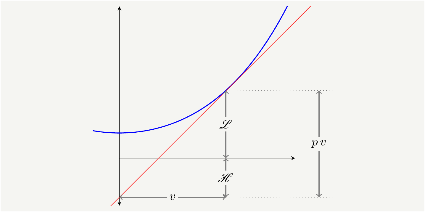
Figure 2: The geometric interpretation of the Legendre transform [3]. The blue curve is the function of interest, \(\mathscr{L}(v)\). The red line is the derivative at point \(v\), which we called \(p(v)\). From the geometry, we have \(\mathscr{L}(v)+\mathscr{H}(p)=p\, v.\)

As seen from the geometry, the original function \(\mathscr{L}\) and the transformed function \(\mathscr{H}\) add up to \(p v\). Therefore we can define the transformation mapping as \[\begin{eqnarray} \{\mathscr{L},v\} \iff \{ \mathscr{H},p\} \tag{16}, \end{eqnarray}\] with the explicit transformation rule as:

\[\begin{eqnarray} \mathscr{L}(v)+\mathscr{H}(p)=p\, v \tag{17}. \end{eqnarray}\]

Geometric derivation using areas

Since there is a one to one map between \(v\) and \(p\), we can plot the functions \(p(v)\) or \(v(p)\), and construct Fig. 3 [2].

Figure 3: The geometric interpretation of the Legendre transform interms of the areas [2]. The red line is \(p(v)\). Since there is a one to one map between \(v\) and \(p\), we can compute the areas using horizontal slices or vertical slices. Since the areas add up to the are of the rectangle, we have \(\mathscr{L}(v)+\mathscr{H}(p)=p\, v\).

The shaded areas can be calculated using horizontal slices or vertical slices as follows: \[\begin{eqnarray} \mathscr{L}(v)\equiv\int_0^v d\tilde v p(\tilde v),\quad \text{and}\quad \mathscr{H}(p)\equiv\int_0^p d\tilde p v(\tilde p) \tag{18}. \end{eqnarray}\] As the areas add up to the area of the rectangle, we have

\[\begin{eqnarray} \mathscr{L}(v)+\mathscr{H}(p)=p\, v, \tag{19} \end{eqnarray}\] which is nothing but the definition of the Legendre transform. Furthermore, we can take the derivatives of the functions in Eq. (18) with respect to their arguments to get:

\[\begin{eqnarray} \frac{\partial \mathscr{L}}{\partial v}= \frac{\partial }{\partial v}\left(\int_0^v d\tilde v p(\tilde v)\right)=p(v),\nonumber\\ \frac{\partial \mathscr{H}}{\partial p}= \frac{\partial }{\partial p}\left(\int_0^p d\tilde p v(\tilde p)\right)=v(p) \tag{20} \end{eqnarray}\] which recovers the original definition of \(p\) in in Eq. (15) and the first part of the Hamiltonian equations of motion in Eq. (12) with \(v=\dot q\).

If we want to recover the other part of the Hamiltonian equations, we need to expose the other argument of \(\mathscr{L}\) and \(\mathscr{H}\), that is \(\mathscr{L}=\mathscr{L}(v,q)\) and \(\mathscr{H}=\mathscr{H}(p,q)\). But note that \(q\) is a totally independent variable. Taking the derivative of Eq. (19) with respect to \(q\), we get:

\[\begin{eqnarray} \frac{\partial \mathscr{L}(v,q) }{\partial q}+\frac{\partial \mathscr{H}(p,q)}{\partial q}=\frac{\partial (pv)}{\partial q}=0 \implies \frac{\partial\mathscr{H}(p,q) }{\partial q}=-\frac{\partial \mathscr{L}(v,q)}{\partial q}=-\dot p, \tag{21} \end{eqnarray}\] where we used Euler’s equation of motion in Eq. (6) to convert \(\frac{\partial \mathscr{L}(v,q)}{\partial q}\) to \(\dot p\).

Inverse Legendre transform

Ever heard of the inverse Legendre transform? Probably not. That is because there is no need to define the inverse transform since it is its own inverse! The definition of the transform in Eq. (19) manifestly shows this: the original function and the transformed one are added to give \(p v\). In other words, we can swap \(\mathscr{L}\) with \(\mathscr{H}\) and \(v\) with \(p\), and nothing will change. Equivalently, we can try to transform \(\mathscr{H}(p)\) one more time. Let’s do that. Remember that we trade the argument of the function with the derivative of the function:

\[\begin{eqnarray} u(p)=\frac{\partial \mathscr{H}}{\partial p}, \tag{22} \end{eqnarray}\] and define the transformed function

\[\begin{eqnarray} \mathscr{H}_2(u)=u p -\mathscr{H}(p) \tag{23}. \end{eqnarray}\] However, from the Hamiltonian equations of motion, we already know that \(u(p)=\frac{\partial \mathscr{H}}{\partial p}=v\). Plugging this back in gives

\[\begin{eqnarray} \mathscr{H}_2(v)=v p -\mathscr{H}(p) \tag{24}, \end{eqnarray}\] and we explicitly see that \(\mathscr{H}_2(v)=\mathscr{L}(v)\), i.e., transforming for the second time undoes the first one and returns back the original function \(\mathscr{L}\).

Extended Lagrangian and Hamiltonian

We have carefully stressed that there is only one independent variable in the game: \(p\) or \(v\) (ignoring the spectator variable \(q\)). The relation between \(p\) and \(v\) is dictated by physics, such as \(p=mv\) for a non-relativistic particle or \(p=\frac{m v}{\sqrt{1-v^2/c^2}}\) for the relativistic one, where \(m\) is the mass of the particle, and \(c\) is the speed of light. However, we can still let \(v\) and \(p\) go off-shell and be independent of each other [4]. This formalism extends the Lagrangian and Hamiltonian into a larger phase-space. The extended functions are defined as [5] \[\begin{eqnarray} \mathscr{H}_e(p,\dot q,q)\equiv p \dot q -\mathscr{L}(\dot q,q)\nonumber\\ \mathscr{L}_e(\dot q,p,q)\equiv p \dot q -\mathscr{H}(p,q) \tag{25}, \end{eqnarray}\] where we switched the notation a bit by defining \(v=\dot q\). Now we treat \(p\) and \(\dot q\) as independent variables, and therefore \(\mathscr{H}_e\) will be a surface. Let us consider a non-relativistic particle of unit mass with with no potential: \(\mathscr{L}(\dot q,q)=\mathscr{L}(\dot q)=\frac{\dot q^2}{2}\). Then the corresponding \(\mathscr{H}_e\) becomes \[\begin{eqnarray} \mathscr{H}_e(\dot q,p,q)\equiv p \dot q -\mathscr{L}(\dot q)= p \dot q -\frac{\dot q^2}{2} \tag{26}, \end{eqnarray}\] which is shown in Fig. 4.

Figure 4: This is an interactive plot: you can hover on it or rotate it. Extended Hamiltonian for a non-relativistic particle [5]. The value of the ordinary Hamiltonian is a slice of the surface, which is the ridge shown in the dashed black line.

We can still recover the original \(\mathscr{H}\) since it is the value of \(\mathscr{H}_e\) when \(p=\dot q\) and it is the ridge of the surface shown with the dashed black line. Mathematically, we have \(\mathscr{H}(p)=\mathscr{H}_e(\dot q(p),p)\). More generically we can write the following:

\[\begin{eqnarray} \mathscr{H}(p,q)\equiv \underset{\dot q}{\text{max}}\left( p \dot q -\mathscr{L}(\dot q,q)\right) \tag{27}, \end{eqnarray}\]

where \(\underset{\dot q}{\text{max}}\) means that the equation is evaluated at the value of \(\dot q\) which maximizes the result. Note that this can be used as the definition of the Legendre transform, and in fact it is what mathematicians do. The Legendre transform of a function \(f(x)\) is defined as follows [6]:

\[\begin{eqnarray} f^*(x^*)=\underset{ x\in I}{\sup}\left(x^* x -f(x)\right),\quad x^* \in I^*\tag{28}, \end{eqnarray}\]

where \(\sup\) denotes the supremum, \(I\) and \(I^*\) are the domains of the functions \(f\) and \(f^*\), respectively. The mapping between the quantities we used earlier and the ones in this formal definition is as follows: \(x\sim \dot q\) and \(x^*\sim p\), \(f\sim \mathscr{L}\), and \(f^*\sim \mathscr{H}\).

This completes our deep dive into the Legendre transform!