Introduction

Qiskit is a Python-based, open-source framework for quantum computing. It supports superconducting qubits and trapped ions as physical implementations. The qiskit library is available at GitHub [1]. This post is a detailed exploration of one of the examples [2] included the qiskit tutorials. All the credit for the code belongs to the qiskit team, and I made only small changes. If you would like to run the original code online, I pulled it into a binder page [3].

The installation of the library is as easy as any other:

pip install qiskit

Once you install the library, you can start playing with the code.

Let the code begin

We load the library and initiate a quantum system of \(3\) qubits.

import numpy as np #
from qiskit import *
circ = QuantumCircuit(3) # Create a Quantum Circuit acting on a quantum register of three qubits

The sequence of operations is as follows:

1. A Hadamard gate on qubit \(0\),
2. A controlled-Not operation (\(C_{X}\)) between qubit \(0\) and qubit \(1\), and
3. A controlled-Not operation between qubit \(0\) and qubit \(2\), as implemented in the code snippet below.

circ.h(0)     # Add a H gate on qubit 0, putting this qubit in superposition.

circ.cx(0, 1) # Add a CX (CNOT) gate on control qubit 0 and target qubit 1, putting the qubits in a Bell state.

circ.cx(0, 2) # Add a CX (CNOT) gate on control qubit 0 and target qubit 2, putting the qubits in a GHZ state.

circ.draw('mpl') # draw the circuit

Qiskit has a specific way of ordering qubits in the state representation. For example, if qubit zero is in state \(0\), qubit \(1\) is in state \(0\), and qubit \(2\) is in state \(1\), Qiskit would represent this state as \(|100\rangle\), compared to typical physics textbook representation of \(|001\rangle\). In this representation, the controlled-not operator, with qubit \(0\) being the control and qubit \(1\) being the target, reads: \[\begin{equation} C_X = \begin{pmatrix} 1 & 0 & 0 & 0 \\ 0 & 0 & 0 & 1 \\ 0 & 0 & 1 & 0 \\ 0 & 1 & 0 & 0 \\\end{pmatrix}\tag{3}. \end{equation}\]

Simulation with Qiskit Aer

Qiskit Aer is the quantum circuits simulating package. It provides various backends for simulations. We will use statevector_simulator. It computes and returns the quantum state. Note that the dimensionality of the state grows exponentially: with \(n\) qubits the result is a complex vector of dimension \(2^n\).

from qiskit import Aer # Import Aer
backend = Aer.get_backend('statevector_simulator') # Run the quantum circuit on a statevector simulator backend
job = execute(circ, backend)# Create a Quantum Program for execution 
result = job.result()# Create a Quantum Program for execution 

The result object contains the data and Qiskit provides the method result.get_statevector(circ) to return the state vector for the quantum circuit.

outputstate = result.get_statevector(circ, decimals=3)
print(outputstate)

## [0.707+0.j 0.   +0.j 0.   +0.j 0.   +0.j 0.   +0.j 0.   +0.j 0.   +0.j
##  0.707+0.j]

The visualization function can be used to plot the real and imaginary components of the state density matrix \(\rho\), which is defined as: \[\begin{equation} \rho\equiv |\psi\rangle\langle\psi|=\frac{|000\rangle\langle 000|+|000\rangle\langle 111|+|000\rangle\langle 000|+|111\rangle\langle 111| }{2}\tag{4}. \end{equation}\]

from qiskit.visualization import plot_state_city
plot_state_city(outputstate)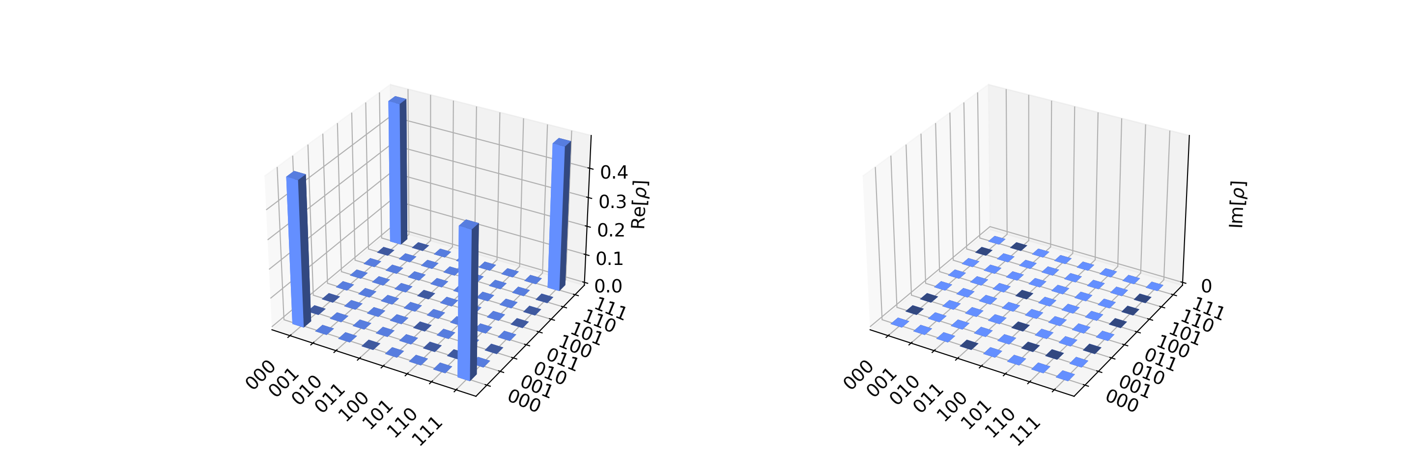

Figure 1: The real and imaginary components of the density matrix. Note that the coefficients are in agreement with the state \(\rho\) as defined in Eq. (4).

Measurement

To simulate a circuit that includes measurement, we add measurements to the original circuit above, and use a different Aer backend.

meas = QuantumCircuit(3, 3)# Create a Quantum Circuit
meas.barrier(range(3))

meas.measure(range(3), range(3))# map the quantum measurement to the classical bits

qc = circ + meas# The Qiskit circuit object supports composition using the addition operator.

The measurement collapses the quantum states onto classical bits. and they are stored in classical registers,

The measurement can be simulated in qasm_simulator. The shots parameter sets the number of simulations.

backend_sim = Aer.get_backend('qasm_simulator')# Use Aer's qasm_simulator
nshots=1024
job_sim = execute(qc, backend_sim, shots=nshots)# Execute the circuit on the qasm simulator.
result_sim = job_sim.result()# Grab the results from the job.

get_counts(circuit) returns aggregated binary outcomes of the simulated circuit

counts = result_sim.get_counts(qc)
p=counts['000']/nshots
print(counts)

## {'000': 517, '111': 507}

plot_histogram can be used to plot the distribution of the outcomes.

from qiskit.visualization import plot_histogram
plot_histogram(counts)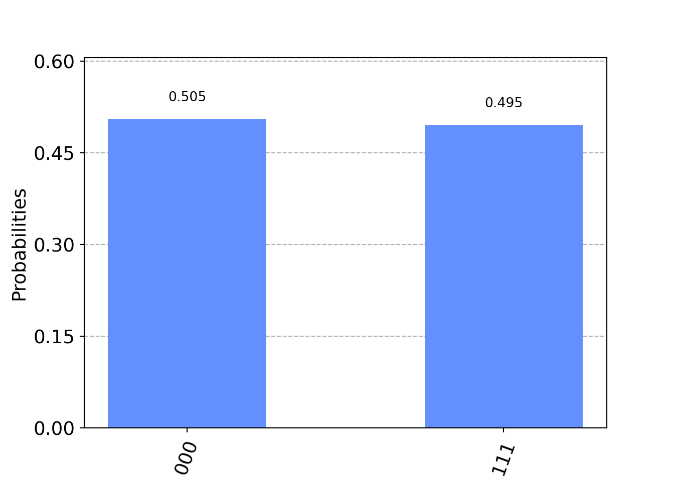

Figure 2: The histogram of the outcomes.

From the output numbers, one can see that 50.5% of the time, we get the classical output \(000\). However, it is always a good practice to compute and include the confidence intervals, say \(95\%\). For a binary random variable, the confidence intervals are given by

\[\begin{equation} \hat p\pm z\sqrt{\frac{\hat p(1-\hat p)}{n_\text{trials}}} \tag{5}, \end{equation}\] where \(\hat p\) is the observed value of the probability and \(z\) is the z-score for the confidence level (i.e., \(1.96\) for \(95\%\)).

delta=1.96*np.sqrt(p*(1-p)/nshots)
pmin=p-delta
pmax=p+delta

Therefore, the simulations with \(1024\) trials show that the probability of measuring state \(000\) is \([ 0.47 , 0.54 ]\) with \(95\%\) confidence.