Probability and entropy

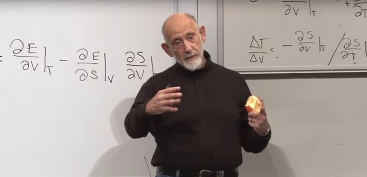
Consider a random variable \(X\) with possible outcomes \(x\). We will want to keep things simple first and consider the case of discrete case, for which there are finite number of outcoumes that we can labels as \(\{x_1,x_2,\cdots, x_N\}\) where \(N\) is the number of possible outcomes. For example, if we are flipping a coin \(N=1\) and \(\{x_1,x_2\}=\{\text{heads},\text{tails} \}\); if we are rolling a die, \(N=6\) and \(\{x_1,x_2,x_3,x_4,x_5, x_6\}=\{1,2,3,4,5,6\}\). We can also assign a probability to observe the outcome \(x_i\) as follows: \[\begin{eqnarray} p_i\equiv P(X=x_i), \tag{1} \end{eqnarray}\] with the unit normalization \[\begin{eqnarray} \sum_{i=1}^N p_i\equiv 1. \tag{2} \end{eqnarray}\] The entropy associated with random variable is a measure of uncertainty in the outcome. Let us consider a uniform distribution as shown in Fig. @ref(fig:uniform.)

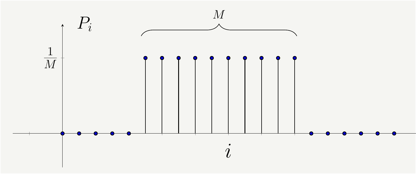
Figure 1: A probablity distribution with \(N\) states, \(M\) of which are possible with probability \(\frac{1}{M}\)

For such a distribution, all the outcomes are equally likely and there are \(N\) of them. The entropy of such a distribution is defined as the logarithm of the number of possible outcomes, that is: \[\begin{eqnarray} S=log(M). \tag{3} \end{eqnarray}\] For a generic distribution, we have to modify this definition. It will be modified as follows: \[\begin{eqnarray} S=-\sum_i p_i \log(p_i). \tag{4} \end{eqnarray}\] We can quickly see that Eq. (4) reduces back to Eq. (3) when \(p_i=\frac{1}{M}\): \[\begin{eqnarray} S=-\sum_i p_i \log(p_i)=-\sum_i \frac{1}{M} \log\left(\frac{1}{M}\right)=-M \frac{1}{M} \log\left(\frac{1}{M}\right)= log(M). \tag{5} \end{eqnarray}\] In order to get to the bottom of this definition in Eq. (4), we have a couple of options, as discussed below.

Defining the entropy

This derivation comes from the father of the information theory, Claude Shannon in his ground breaking paper[1]. We define an information function, \(H\), which takes in the probability distribution, i.e., \(H=H(p_1,p_2, \cdots,p_N)\). Shannon requires the following features in \(H\) :

1. \(H\) should be continuous in the \(p_i\).
2. If all \(p_i\) are equal, \(p_i=1/N\), then \(H\) should be a monotonically increasing function of \(n\). With equally likely events there is more choice, or uncertainty, when there are more possible events.
3. The total information extracted from two events must be the sum of the information collected from each: \(H(p\times q)=H(p)+H(q)\).

You can clearly see that the third requirement is begging for a \(log\) function, i.e. \(H(p)=-log(p)\). Shannon shows that it is the only function that meets all of the requirements. Note that the negative sign in front of Eq. (4) makes sure the second requirement is satisfied. For multiple \(p_i\), we simply sum over \(p_i\)’s.

There is another way of getting the same answer by combinatorics. Let us assume that we have

Another way of getting the same result is by using the Stirling’s approximation for factorial. Consider a stream of \(n\) bits consisting of \(0\)’s and \(1\)’s. If the probability of a bit being \(1\) is \(p\), for large \(n\), the average number of \(1\)’a in such messages will be \(n p\), and the average number of \(0\)’s will be \(n(1-p)\). We can easily estimate the number of different messages that can me constructed with these many \(0\)’s and \(1\)’s as \(\binom{n}{np}\) , and compute its log:

\[\begin{eqnarray} log\binom{n}{np}&=&\frac{n!}{np!\, n(1-p)!}\simeq n log (n) -n -np \,log(np) +np -n(1-p)\,log\left( n(1-p)\right)+n(1-p)\nonumber\\ &=&-n \left[p\, log(p)+ (1-p)\,log(1-p) \right],\tag{6} \end{eqnarray}\] where we used the Stirling approximation \(log(n!)=n\, log(n)-n+ \mathcal{O}(log(n))\).

Derivation of the Stirling formula Hide

Consider the following integral: \[\begin{eqnarray} \int_0^\infty dx x^{n}e^{-x}= \left[(-1)^n\frac{d^n}{d\alpha^n}\int_0^\infty dx e^{-\alpha x}\right]_{\alpha=1} =\left[(-1)^n\frac{d^n}{d\alpha^n} \frac{1}{\alpha}\right]_{\alpha=1}=n!. \tag{7} \end{eqnarray}\] Taking this definition, we can do the following: \[\begin{eqnarray} n!=\int_0^\infty dx x^{n}e^{-x}=\int_0^\infty dx e^{n ln(x)-x}. \tag{8} \end{eqnarray}\] Let’s take a close look at the function in the exponent: \[\begin{eqnarray} u(x) &=&n ln(x)-x, \tag{9} \end{eqnarray}\] as shown in Fig. 2. This function has its peak value at \(x=n\). Note that this function appears in the exponent, under the integral. The dominant contribution to the integral will come from the domain around \(x=n\). we can expand \(u(x)\) around \(x=n\):

\[\begin{eqnarray} u(x) &=&n ln(x)-x =n ln(x-n +n)-x=n ln(n[1 +\frac{x-n}{n}])-x\nonumber\\ & \simeq& n \left( ln(n)+\frac{x-n}{n} -\frac{1}{2}\left[\frac{x-n}{n}\right]^2 \right)-x =n ln(n) -n -\frac{1}{2}\frac{(x-n)^2}{n}\equiv \tilde{u}(x). \tag{10} \end{eqnarray}\]

The original function and the approximated functions are plotted in Fig. 2.

\(n\)

Figure 2: Interactive plot showing \(u(x)\) (left), \(e^{u(x)}\), and \(e^{\tilde{u}(x)}\) (right).

From Fig. 2, we also notice that if we extended the \(x\) range to include negative values, the integral would not change much since \(e^{\frac{1}{2}\frac{(x-n)^2}{n}}\) is rapidly decaying. Therefore we can change the lower limit of the integral from \(0\) to \(-\infty\) to get:

\[\begin{eqnarray} n!&=&\int_0^\infty dx x^{n}e^{-x}=\int_0^\infty dx e^{u(x)}\simeq \int_0^\infty dx e^{\tilde{u}(x)}=n^n e^{-n} \int_0^\infty dx e^{-\frac{1}{2}\frac{(x-n)^2}{n}}\nonumber\\ &\simeq&n^n e^{-n} \int_{-\infty }^\infty dx e^{-\frac{1}{2}\frac{(x-n)^2}{n}}=n^n e^{-n} \sqrt{2\pi n}=\sqrt{2\pi n}\left(\frac{n}{e}\right)^n. \tag{11} \end{eqnarray}\]

Figure 3 shows the comparison of \(n!\) with the Stirling’s approximation given in Eq. (11).

Figure 3: The plot of \(n!\) and its Stirling’s approximation (left). The relative error(right) gets smaller as \(n\) increases.

Figure 4: The entropy: \(S(p)\), is maximized when \(p=\frac{1}{2}\).

Equation (4) has a summation since we assumed discrete distribution specified by index \(i\). The continuous version of it is straight forward to write: \[\begin{eqnarray} S=-\int dx p(x) \log\left(p(x)\right), \tag{12} \end{eqnarray}\] where the integral is evaluated over the space \(p(x)\) is defined. What kind of distribution would maximize the entropy? One can anticipate that it has to be the uniform distribution defined in a specific range. And we can easily prove that using calculus of variations with Lagrange multipliers. The Lagrange multiplier comes in to satisfy the normalization of the probability density, similar to Eq. (2) \[\begin{eqnarray} \int dx p(x) =1. \tag{13} \end{eqnarray}\]

More about Lagrange multipliers Hide

In optimization problems with constraints, one tries to find the extrema of a function while satisfying the contraints imposed. Consider a function, \(f(x,y)\), and assume we want to find the location \((x_0,y_0)\) for which \(f(x_0,y_0)\) assumes its maximum, and at the same time we want a constrain function to be satisfies: \(g(x_0,y_0)=0\). One can solve this problem using brute force:

• Require \(\mathbf{\nabla} f(x,y)\vert_{(x_0,y_0)}=0\) and \(g(x_0,y_0)=0\).
• Solve these two equations with two unknowns.

Although it is technically possible to solve it this way, it may require us to invert complicated functions which might be hard to do. It gets even harder as we introduce more variables and constraints. We can do better than that!

Let us consider a contour curve of \(f\), which is the pairs of numbers \((x,y)\) for which \(f(x,y)=k\). We want \(k\) to be as large as possible while satisfying \(g(x_0,y_0)=0\). To illustrate the method, let us take the following functions:

\[\begin{eqnarray} f(x,y)=y^2-x^2, \quad g(x,y)=x^2+y^2-1, \tag{14} \end{eqnarray}\] which are shown in Fig. 5.

\(k\)

Figure 5: Showing the \(x,y\) values satisfying \(f(x,y)=k\), and the constraint function \(g(x,y)=x^2+y^2-1=0\), which is the unit circle. You can change the value of \(k\) and observe how the curve moves. Also follow the slopes of the curves at one of the intersection points.

If there was no constraint, we would increase the value of \(k\) indefinitely. However, we are required to find a solution \((x_0,y_0)\) that satisfies \(g(x_0,y_0)=0\), which means two curves have to pass through the point \((x_0,y_0)\). As you tune the value of \(k\), you realize that you can make the curves to intersect at different points. The optimal solution is the one at which two curves touch each other, and, for this particular example, we can graphically see that it happens at \(k=1\) and \((x_0,y_0)=(0,1)\).

How do we solve this analytically though? Note that in this critical point, two curves are barely touching each other. More precisely, they are tangent to each other at that point, i.e., they have the same value and the same slope. Since the tangents are the same, the vector which is perpendicular to the tangents must be the same too. And that perpendicular vector is nothing but the gradient. Note that we are limiting ourselves to a two-dimensional problem for pedagogical reasons. The observation above holds for any dimension. Let’s prove that gradient vector is indeed perpendicular to the curve. In a generic case, \(f\) can be a function of multiple variables: \(f=f(x_1,x_2,\cdots,x_n)\) where \(\mathbf{x}=(x_1,x_2,\cdots,x_n)\) is an \(n\) dimensional vector. The level surface of this function is composed of \(\mathbf{x}\) values such that \(f(\mathbf{x}_0)=k\), which defines an \(n-1\) dimensional level surface. What we want to prove is that for any point on the level surface, \(f(\mathbf{x}_0)=k\), the gradient of \(f\), i.e., \(\mathbf{\nabla}f\vert_{\mathbf{x}_0}\) is perpendicular to the surface.

Let us take an arbitrary curve on this surface, \(\mathbf{x}(t)\), parameterized by a parameter \(t\), and assume it passes through \(\mathbf{x}_0\) at \(t=t_0\). On the surface \(f(\mathbf{x}(t))=f\left(x_1(t),x_2(t),\cdots,x_n(t)\right)= k\). Let’s take the parametric derivative of \(f\) and apply the chain rule.

\[\begin{eqnarray} \frac{df}{dt}=0=\sum_{i=1}^n \left.\frac{\partial f}{\partial x_i}\right\vert_{\mathbf{x}_0}\left. \frac{d x_i}{dt}\right\vert_{t_0} = \left.\mathbf{\nabla} f\right\vert_{\mathbf{x}_0} \cdot \dot{\mathbf{x}}\vert_{t_0} \tag{15}, \end{eqnarray}\] where we defined \(\dot{\mathbf{x}}\vert_{t_0}=\left.\frac{d\mathbf{x}(t)}{dt}\right\vert_{t_0}\), which is nothing but the tangent line. Therefore we conclude that the gradient is perpendicular to the tangent lines on the surface.

This exercise tells us that the gradients of the function we want to optimize is parallel to the gradient of the constraint function. That is:

\[\begin{eqnarray} \left.\mathbf{\nabla} f \right\vert_{\mathbf{x}_0}= \lambda \left.\mathbf{\nabla} g\right\vert_{\mathbf{x}_0}\tag{16}, \end{eqnarray}\] where the constant \(\lambda\) is the Lagrange multiplier. And keep in mind that we also need to satisfy \(g(\mathbf{x}_0)=0\) We can neatly combine these to requirements by defining a new function:

\[\begin{eqnarray} h(\mathbf{x},\lambda)= f(\mathbf{x}) -\lambda g(\mathbf{x})\tag{17}, \end{eqnarray}\] which can be optimized by requiring

\[\begin{eqnarray} \left.\mathbf{\nabla} h\right\vert_{\mathbf{x}_0}=0, \quad \text{and}\quad \left.\frac{\partial h}{\partial \lambda}\right\vert_{\mathbf{x}_0}=0 \tag{18}. \end{eqnarray}\] The bottom line is that the constraint itself is mixed into the function that we want to optimize. The expression in (18) has equal number of equations and unknowns, so we can solve for \(\mathbf{x}_0\) and \(\lambda\).

See this post for examples.

Combining the condition with the target function to maximize, Eq. (12), we have the following integral to maximize: \[\begin{eqnarray} I=-\int dx p(x) \log\left(p(x)\right)-\lambda\left( \int dx p(x)-1 \right)=- \int dx p(x) \left( \log\left(p(x)\right) +\lambda \right)+\lambda \tag{19} \end{eqnarray}\]

Now move the function \(p(x)\) to \(p(x)+\delta(x)\), and require that \(\delta I=0\) for the \(p(x)\) that maximizes \(I\). This yields: \[\begin{eqnarray} \delta I=-\int dx \delta p(x) \left[ \log\left(p(x)\right)+1 +\lambda \right]=0. \tag{20} \end{eqnarray}\] Since \(\delta p(x)\) is totally arbitrary, we need \(\log\left(p(x)\right)+1 +\lambda=0\). Furthermore, as \(\lambda\) is just a constant, this shows that \(p(x)\) is also a constant. Let’s assume that we are interested in distributions defined in the range \([a,b]\). The normalization condition in Eq. (13) uniquely defines the value of the constant as \(\frac{1}{b-a}\).

The laws of thermodynamics

So far we have been talking about probability distributions in the most abstract form. They can be anything: coin flip, bits in a message to be transmitted etc. Let’s now switch to physical cases. In such cases, the probability distributions will be parameterized by a physical quantity, such as the average energy \(E\). \[\begin{eqnarray} S(E)=-\sum_i p_i \log\left(p_i\right), \tag{21} \end{eqnarray}\] where we are using the discrete index \(i\) and the sum. The average value of energy, \(E\) is the statistical average: \[\begin{eqnarray} E=\sum_i p_i E_i, \tag{21} \end{eqnarray}\] where \(E_i\) is the energy values of the state \(i\), and the probability of that state to be occupied is \(p_i\). It is emphasize again that \(E\) is the average energy of the system, and it would have been more appropriate to denote it as \(\bar{E}\) or \(\langle E\rangle\), however, that would look very ugly in the equations. We will keep it as \(E\) and promise to remember that it is the mean value of the energy, not the energy of each level or particle. This might look recursive, but it will make more sense as we proceed.

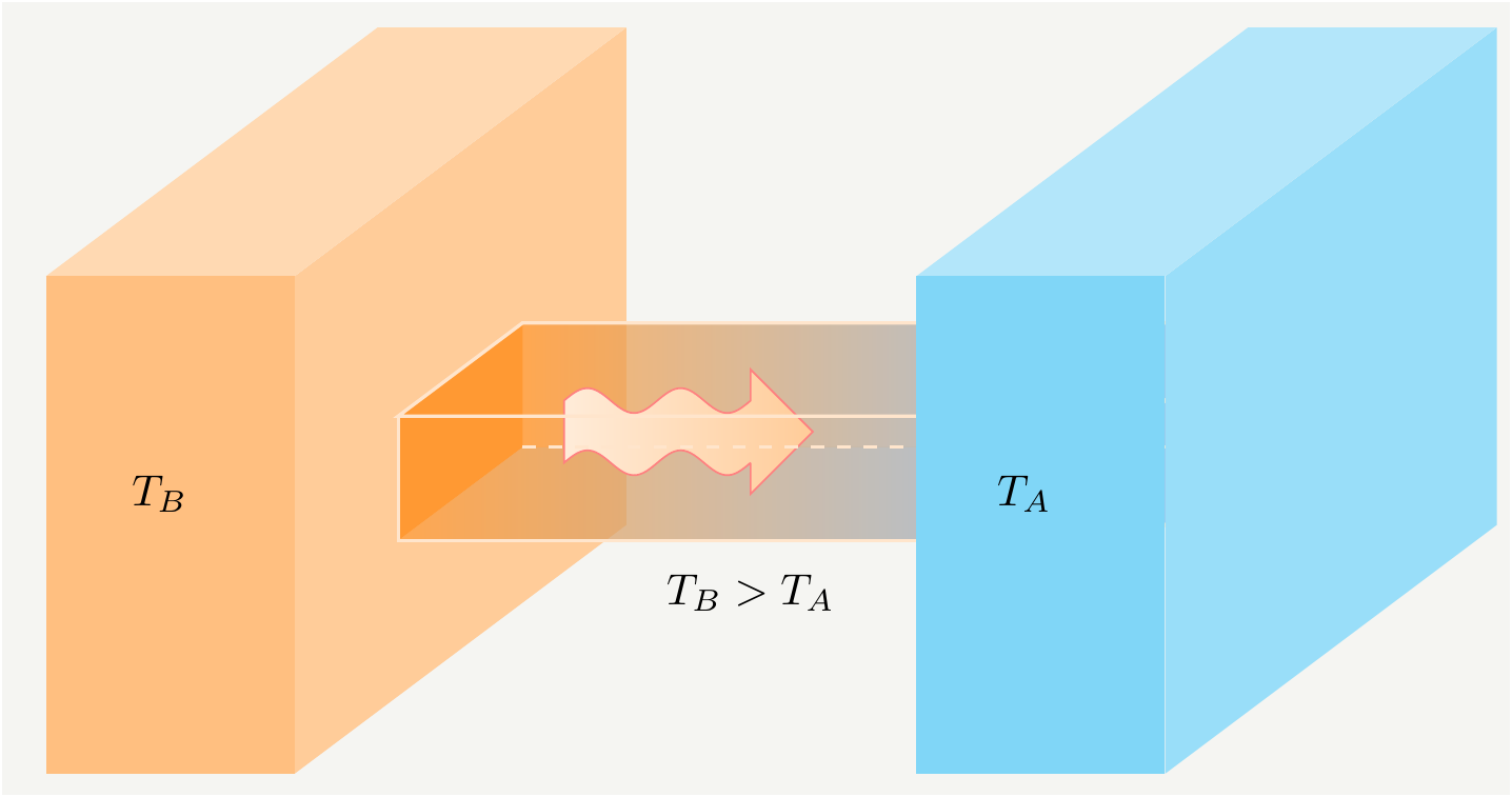
Figure 6: Two containers at temperatures \(T_B\) and \(T_A\) with \(T_B>T_A\) are connected to exchange heat.

Let us state the first and second law:

• \(1^\text{st}\) law of thermodynamics: Energy is conserved.
• \(2^\text{st}\) law of thermodynamics: Entropy always increases.

The total entropy of the system is given by the sum of the entropies of the subsystems: \[\begin{eqnarray} S=S_A+S_B. \tag{22} \end{eqnarray}\] The first law implies that changes in energies add up to zero: \[\begin{eqnarray} dE_A+dE_B=0. \tag{23} \end{eqnarray}\]

The second law requires: \[\begin{eqnarray} dS=dS_A+dS_B>0 \tag{24} \end{eqnarray}\]

The temperature of a system is defined in terms of the entropy function \(S(E)\) as follows: \[\begin{eqnarray} T\equiv\frac{dE}{dS}. \tag{25} \end{eqnarray}\] Inserting the definition from Eq. (25) into Eq. (23) we get:

\[\begin{eqnarray} dE_A+dE_B=0= T_A dS_A+T_Bd S_B \implies dS_B=-\frac{T_A}{T_B }d S_A. \tag{23} \end{eqnarray}\] Putting this in the second law in Eq. (24), we get

The second law requires: \[\begin{eqnarray} dS=dS_A+dS_B= \left(1-\frac{T_A}{T_B} \right)dS_A=T_B(T_B-T_A)dS_A >0. \tag{24} \end{eqnarray}\] Since \(T_B>0\) and \(T_B>T_A\), we conclude that \(dS_A>0\), that is entropy increases. Also note that \(T_AdS_A=dE_A>0\), therefore the energy is flowing to container \(A\) from \(B\). As \(T_B\) equalizes with \(T_A\), the heat flow will stop and two containers will be in equilibrium. Therefore it is the temperature that determines the direction of the energy. One can extend the analysis above to a third container to state the \(0^\text{th}\) law od thermodynamics:

• \(0^\text{th}\) law of thermodynamics: If two systems are both in thermal equilibrium with a third system, then they are in thermal equilibrium with each other.

Occupation number

Consider a system with \(m\) states. An occupation number is the number of systems, \(n\), occupying a given \(i^\text{th}\) state, and we will denote this number as \(n_i\). Given \(m\) such states, i.e., \(i\in\{1,2,\cdots,m\}\), we are interested in finding the total number of possible ways to redistribute the systems among the states. This is illustrated in Fig. 7.

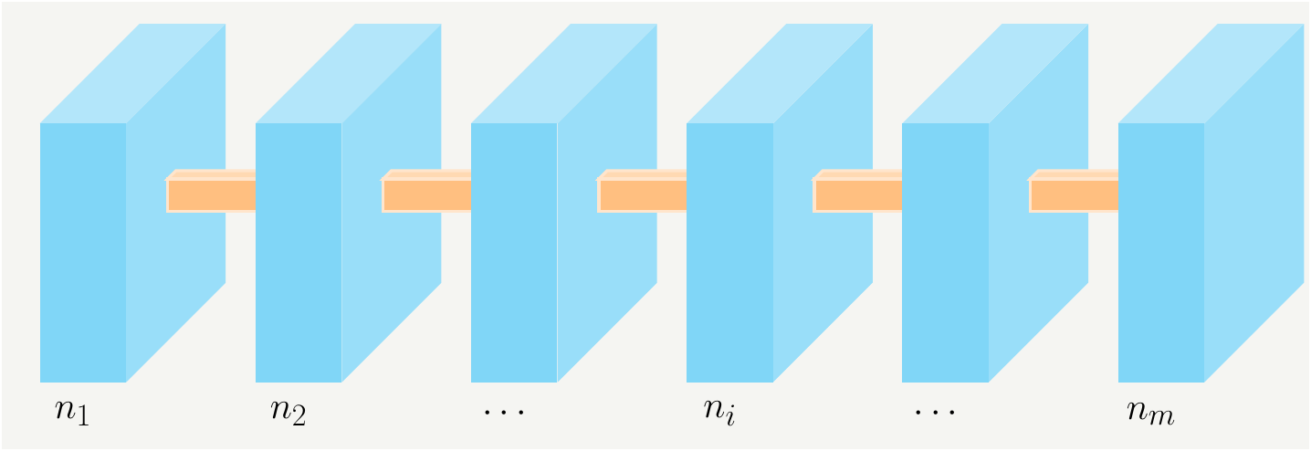
Figure 7: \(m\) boxes with given occupation numbers \(n_i\).

We assume that the total number of occupation number is fixed, we will define it as \(N\): \[\begin{eqnarray} N\equiv\sum_{i=1}^m n_i. \tag{26} \end{eqnarray}\] For a randomly selected system, the probability of that system to be in state \(i\) is the ratio of the number of states in the \(i^\text{th}\) and the total number of states: \[\begin{eqnarray} p_i= \frac{n_i}{N}, \tag{1} \end{eqnarray}\] which results in a normalized probability distribution: \[\begin{eqnarray} \sum_{i=1}^m p_i= 1. \tag{27} \end{eqnarray}\] We also need to make sure that total energy is conserved: \[\begin{eqnarray} \sum_{i=1}^m E_i n_i =N \sum_{i=1}^m E_i \frac{n_i}{N} =N\sum_{i=1}^m E_i p_i=N E, \tag{28} \end{eqnarray}\] where \(E\) is the average energy. While keeping the occupation numbers fixed, we can shuffle systems around to create different configurations. For \(N\) systems, we get \(N!\) shufflings. However, we should remove the overcounting within the states with \(n_i\) as the occupation number. Therefore the total number of combination to create such as system is: \[\begin{eqnarray} C= \frac{N!}{\prod_{i=1}^{m} n_i!}. \tag{29} \end{eqnarray}\] We can now take the log of \(C\) and use the Stirling approximation: \(n!=\sqrt{2\pi n}\left(\frac{n}{e}\right)^n\): \[\begin{eqnarray} log(C)&=& log(N!)-\sum_{i=1}^mlog(n_i!)=N log(N)-N-\sum_{i=1}^mnilog(n_i)+\sum_{i=1}^mn_i+\mathcal{O}(1)\nonumber\\ &=&-N \sum_{i=1}^m\frac{ni}{N}log\left(\frac{ni}{N}\right)=-N\sum_{i=1}^m p_i log(p_i). \tag{30} \end{eqnarray}\] We have shown earlier that this expression is maximized when \(p_i\) are equally likely, which was the case for the Shannon entropy. However, it is very different for this case since we have an additional constraint now, as described in Eqs. (26) and (27). We will multiply these constraints with Lagrange multipliers which we will call \(\alpha\) and \(\beta\), and subtract them from the original function in Eq. (30). Therefore the combined function becomes: \[\begin{eqnarray} h(p_i,\alpha,\beta) &=& -N \sum_{i=1}^m p_i log(p_i)- \alpha\left(\sum_{i=1}^m n_i-N \right) - \beta\left(N \sum_{i=1}^m E_i p_i -N E \right)\nonumber\\ &=&-N\left\{ \sum_{i=1}^m p_i log(p_i)- \alpha\left(\sum_{i=1}^m p_i-1 \right) - \beta\left( \sum_{i=1}^m E_i p_i - E \right) \right\} \tag{31} \end{eqnarray}\] Note that overall factors, such as the factor \(N\) in Eq. (31), do not affect the optimization. Now we just do the math: \[\begin{eqnarray} \frac{\partial}{\partial p_j }h(p,\alpha,\beta) &=& 0= - log(p_j)-1 - \alpha - \beta E_j \tag{32} \end{eqnarray}\] which implies \[\begin{eqnarray} p_j=e^{-\left(1+\alpha+\beta E_j \right)}=e^{-\left(1+\alpha \right)}e^{-\beta E_j }\equiv \frac{e^{-\beta E_j }}{\mathcal{Z}}, \tag{33} \end{eqnarray}\] where \[\begin{eqnarray} \mathcal{Z}\equiv e^{1+\alpha}. \tag{34} \end{eqnarray}\] \(\mathcal{Z}\) is referred to as the partition function, and one can think of it as the normalization factor. We can see that by imposing the normalization condition in Eq. (27): \[\begin{eqnarray} \sum_{i=1}^m p_i= 1=\sum_{i=1}^m \frac{e^{-\beta E_i }}{\mathcal{Z}}, \tag{35} \end{eqnarray}\] which results in: \[\begin{eqnarray} \mathcal{Z}=\sum_{i=1}^m e^{-\beta E_i} . \tag{36} \end{eqnarray}\]

We can figure out the relation between \(\mathcal{Z}\) and \(E\) by imposing the conservation of energy constraints in Eq. (28): \[\begin{eqnarray} E&=&\sum_{i=1}^m E_i p_i= \sum_{i=1}^m E_i \frac{e^{-\beta E_i }}{\mathcal{Z}}=\frac{1}{\mathcal{Z}}\sum_{i=1}^m E_i e^{-\beta E_i } =\frac{1}{\mathcal{Z}}\left(-\frac{\partial }{\partial \beta}\right) \left[\sum_{i=1}^m e^{-\beta E_i } \right]\nonumber\\ &=&-\frac{1}{\mathcal{Z}}\frac{\partial \mathcal{Z} }{\partial \beta}= -\frac{\partial log \mathcal{Z} }{\partial \beta}. \tag{37} \end{eqnarray}\] We can now compute the entropy: \[\begin{eqnarray} S&=& -N\sum_{i=1}^m p_i log(p_i)=-N\sum_{i=1}^m \left[ \frac{e^{-\beta E_i }}{\mathcal{Z}} log\left( \frac{e^{-\beta E_i }}{\mathcal{Z}} \right) \right]\nonumber\\ &=& \beta E +log(\mathcal{Z}). \tag{38} \end{eqnarray}\]