Renewal processes and Poisson processes are fundamental concepts in probability theory and stochastic processes, with wide-ranging applications in fields such as queueing theory, reliability engineering, and operations research. A renewal process is a generalization of the Poisson process, where the time between events (inter-arrival times) is not necessarily exponentially distributed [1]. The Poisson process, a special case of renewal processes, is characterized by events occurring continuously and independently at a constant average rate [2]. Arrival times, which represent the moments when events occur in these processes, play a crucial role in analyzing system behavior and performance [3]. Understanding these concepts is essential for modeling and analyzing various real-world phenomena, from customer arrivals at a service center to the occurrence of equipment failures in industrial settings.
One classic example of renewal theory in action is when you’re dealing with things that break or need maintenance. Picture this: you have a component that you install at time 0. It fails at some random time \(T_1\), and you swap it out for a new one. This new component also has a random lifespan \(T_2\), just like \(T_1\), and the cycle continues. If you’re wondering how many times you’ve replaced this thing by time \(t\), you will find the answer in this post.
If you are well versed in statistics, you will know that there are lots of confusion around the Poisson processes. People will call our good old friend, the exponential distribution, a Poisson distribution, for example. Or they will say arrival times are Poisson distributed, or they will say the total time is Poisson distributed. None these are correct; and we will address them all in this post!
However, before we do all that, you may find it usefull to look at an earlier post Musings on Exponential distribution, which is also tucked in under the button below.Many processes in physics are defined by exponential distribution. Have you ever wondered what that is the case? That is because it is the only one available for microscopic systems. A microscopic system, such as a radioactive atom has no internal memory. And the only continuous distribution with no memory is the exponential distribution. Let’ prove this. Consider a random variable \(X\) defined by its probability function \(F_X(x)=P(X\leq x)\), which is read as probability of \(X\) being less than a given number \(x\). Typically \(X\) is associated with some kind of event or failure, and that is why a counter part of \(F_X\) is defined as the survival function \(S_X\) Define the survival function \(S(t)\): \[\begin{eqnarray} S_X(x)=1-F_X(x)=1-P(X\leq x)=P(X> x) \tag{1}. \end{eqnarray}\] What is the conditional probability of \(X>x+s\) given that it survived until \(x\)? \[\begin{eqnarray} P(X>x+s|X>x)=\frac{P(X>x+s)} {P(X>x)}=\frac{S_X(x+s)} {S_X(x)} \tag{2}. \end{eqnarray}\] The critical observation is this: if the process has no memory, the conditional probability can only depend on the difference in observation points. Think about it this way: the probability of an atom to decay before \(t=1\) year given that it is intact at \(t=0\) is the same as the probability of it decaying within \(t=11\) year given that it is intact at \(t=10\) year. Atoms don’t remember how old they are. Therefore we require that the right hand side of Eq. (2) has no \(x\) dependence, that is: \[\begin{eqnarray} \frac{S_X(x+s)} {S_X(x)}=S_X(s) \implies S_X(x+s)=S_X(x) S_X(s), \tag{3} \end{eqnarray}\] which is begging for the exponential function due to its homomorphism property mapping multiplication to addition. To show this explicitly, consider the repeated application of \(S(x)\) \(p\) times \[\begin{eqnarray} \left[S_X(x)\right]^p=\underbrace{S_X(x)S_X(x)\cdots S_X(x)}_{p \text{ times}}=S_X(p x), \tag{4} \end{eqnarray}\] where \(p\) is a natural number. This certainly holds for natural numbers, but we can do better. Now consider another counting number \(q\) and apply \(S(x/q)\) \(q\) times \[\begin{eqnarray} \left[S_X\left(\frac{x}{q} \right)\right]^q=\underbrace{S_X\left(\frac{x}{q} \right) S_X\left(\frac{x}{q} \right)\cdots S_X\left(\frac{x}{q} \right)}_{q \text{ times}}=S_X\left(q \frac{x}{q} \right) =S_X(x)\implies S_X\left(\frac{x}{q} \right)=\left[S_X\left(x \right)\right]^{\frac{1}{q}}. \tag{5} \end{eqnarray}\] Since we can make this work for \(p\) and \(1/q\), it also works for \(p/q\): \[\begin{eqnarray} S_X\left(\frac{p}{q} x\right)=S_X\left(p \frac{x}{q}\right)=\left[S_X\left(\frac{x}{q}\right)\right]^p =\left[\left(S_X(x)\right)^\frac{1}{q}\right]^p =\left[S_X(x)\right]^\frac{p}{q}. \tag{6} \end{eqnarray}\] That is \[\begin{eqnarray} S_X\left(a x\right)=\left[S_X(x)\right]^a, \tag{7} \end{eqnarray}\] where \(a=\frac{p}{q}\) is a rational number. What about irrational numbers? Since the rationals are a dense subset of the real numbers, for every real number we can find rational numbers arbitrarily close to it[4]. The continuity of \(S\) ensure that we can upgrade \(a\) from an rational number to a real number. One last thing to do is to show that we are getting our old friend \(e\) out of this. Setting \(x=1\) in Eq. (7) gives
\[\begin{eqnarray} S_X\left(a\right)=\left[S_X(1)\right]^a =\left(\exp\left\{-\ln\left[S_X(1)\right] \right\}\right)^a\equiv e^{-\lambda a}, \tag{8} \end{eqnarray}\] where \(\lambda=-\ln\left[S_X(1)\right]>0\).
This derivation is very satisfying, particularly for a non-mathematician like me. But it is a bit too rigorous. We can do a physicist version of this derivation. We start from Eq. (3), take the log and the derivative of both sides with respect to \(s\):
\[\begin{eqnarray} \frac{d}{ds}\log \left(S_X(x+s)\right)&=&\frac{S'_X(x+s)}{S_X(x+s)}\nonumber\\ \frac{d}{ds}\log \left(S_X(x) S_X(s)\right)&=&\frac{d}{ds}\left[\log \left(S_X(x)\right) +\log \left(S_X(s)\right)\right]=\frac{S'_X(s)}{S_X(s)}. \tag{9} \end{eqnarray}\] They are equal to each other: \[\begin{eqnarray} \frac{S'_X(x+s)}{S_X(x+s)}=\frac{S'_X(s)}{S_X(s)}\equiv -\lambda, \tag{10} \end{eqnarray}\] where we realized that the terms are functions of \(s\) or \(x+s\), and they cannot possibly be equal to each other unless they are equal to a constant. Integrating, we get:
\[\begin{eqnarray} \frac{S'_X(s)}{S_X(s)}=\frac{d}{ds}\left[\log \left(S_X(s)\right)\right]= -\lambda \implies S_X(s)= e^{-\lambda s} \tag{11}, \end{eqnarray}\] which completes the proof.
One of the difficulties with such proofs is that, they are done backwards. In fact, life would have been much easier if we started from the so called hazard function. I talked about this in one of my earlier posts:
Musings on Weibull distribution. If we start from a hazard function (ratio of failures to the survivors) \(h\) and define everything else on top, this is how things go:
\[\begin{eqnarray}
h(t)& \equiv& \frac{f(t)}{1-F(t)}= \frac{\frac{d}{dt} F(t)}{1-F(t)}=-\frac{d}{dt}\left[ln\left( 1-F(t)\right)\right]
\implies F(t)=1-e^{-\int_0^td\tau h(\tau)}
\tag{12}.
\end{eqnarray}\]
If you go with the simplest assumption (memory-less, constant) \(h=\lambda\), you get the exponential distribution.
Definitions
In this setup, \(T_1, T_2, \ldots\) are your independent, identically distributed, nonnegative random variables representing those random interarrival times. Let us set up the definitions for \(T_i\): \[\begin{eqnarray} F_{T_i}(x)=P(T_i<x) \tag{13}. \end{eqnarray}\] \(T_i\) are the interaarival times, i.e., it is the time difference between the consequentive events, and by definition they are positive definite. The total time until the \(n^\text{th}\) arrival is a simple sum: \[\begin{eqnarray} S_n=\sum_{i=1}^n T_i \tag{14}. \end{eqnarray}\] We can also create a counter that will return the number of arrivals at any given time \(t\): \[\begin{eqnarray} N(t)=\sum_{i=1}^\infty\theta\left(S_i\leq t\right) \tag{15}. \end{eqnarray}\] where \(\theta\) is the standard unit-step function. To avoid any confusion, let’s put all of these definition in Tab. 1,
| Parameter | Relevant Formulas | Description |
|---|---|---|
| \(T_i\) | - | Interarrival time |
| \(S_n\) | \(\sum_{i=1}^n T_i\) | Total wait time until the \(n^\text{th}\) arrival |
| \(N(t)\) | \(\sum_{i=1}^\infty\theta\left(S_i\leq t\right)\) | Total number of arrivals at time \(t\) |
and illustrate them in Fig. 1.
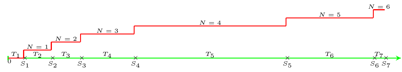
Figure 1: Random events arriving at \(t=S_1,S_2\cdots\). Interarrival times are labeled as \(T_1,T_2\cdots\), and finally \(N=1,2\cdots\) simply counts the arrivals.
\(N(t)\) and \(S_n\) are both random variables. The main goal is to figure out the distribution of \(N(t)\), and we are going to do that in two different ways.
A tedious solution
The set of outcomes with \(N(t)\) will be larger than an integer \(n\) for a given \(t\) is equal to the set of outcomes with \(S_n(t)\) being less than \(t\). That is: \[\begin{eqnarray} \left\{N\geq n\right\}=\left\{S_n\leq t\right\} \implies P\left(N\geq n\right)=P\left(S_n\leq t\right) \tag{16}, \end{eqnarray}\] where we dropped the argument of \(N\) to simplify the notation.
We will use some features of sets. Consider two events \(A\) and \(B\). The probability of \(A\) can be split into two disjoint parts:
- The probability that \(A\) occurs and \(B\) also occurs: \(P(A \cap B)\).
- The probability that \(A\) occurs and \(B\) does not occur: \(P(A \cap B^c)\), which is illustrated in Fig. 2
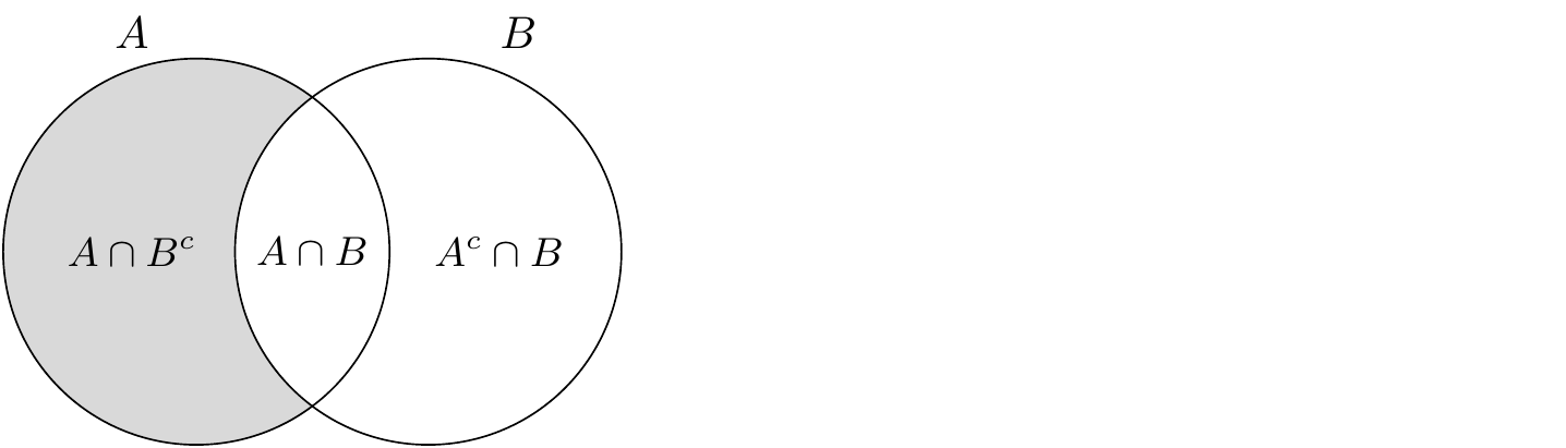
Figure 2: The Venn diagram of the sets \(A\) and \(B\) .
Since these two scenarios cover all possibilities for event \(A\), we can write:
\[\begin{eqnarray} \mathbb{P}(A) &=& \mathbb{P}(A \cap B) + \mathbb{P}(A \cap B^c) \tag{17}, \end{eqnarray}\]
To find the probability of \(A\) intersecting with the complement of \(B\), isolate \(\mathbb{P}(A \cap B^c)\) from the equation:
\[\begin{eqnarray} \mathbb{P}(A \cap B^c) &=& \mathbb{P}(A) - \mathbb{P}(A \cap B) \tag{18}, \end{eqnarray}\]
This equation shows that the probability of \(A\) occurring while \(B\) does not occur is the difference between the probability of \(A\) and the probability that both \(A\) and \(B\) occur together. In our particular case, \(A=\{N\geq n\}\) and \(B=\{N\geq n+1\}\) and \(A\) will be a subset of \(B\). Using this relation we can compute the probability of having exactly \(n\) arrivals at time \(t\): \[\begin{eqnarray} \mathbb{P}\left(N=n\right)=\mathbb{P}\left(N\geq n\right)-\mathbb{P}\left(N\geq n+1\right) \tag{19}, \end{eqnarray}\]
Let’s define the following probability: \[\begin{eqnarray} G_n(t)\equiv \mathbb{P}\left(S_n>t\right)\tag{20}, \end{eqnarray}\] and attempt to calculate it recursively. We first single out one of the events, say \(T_1\) and split the possibilities into two cases:
- Total time, \(S_n\), turns out to be larger than \(t\) simply because \(T_1\) is larger than \(t\).
- Total time, \(S_n\), turns out to be larger than \(t\) because \(T_1\) outcome was \(\tau\) where \(\tau<t\), but the rest of the events added up to a value larger thah \(t-x\), that is \(T_2+\cdots+T_n>t-x\).
Since these two events are mutually exclusive, we can add the individual probabilities to get the total probability: \[\begin{eqnarray} G_n(t)&=& \mathbb{P}\left(S_n>t\right)= \mathbb{P}\left(T_1>t\right)+\int_0^t d\tau f_{T_1}(\tau) \mathbb{P}\left( T_2+T_3+\cdots+T_n>t-\tau\right)\nonumber\\ &=& e^{-\lambda t}+\lambda\int_0^t d\tau e^{-\lambda \tau} G_{n-1}(t-\tau) \tag{21}. \end{eqnarray}\] This is a integral equation and we can attempt to solve it by a series expansion with the following trial function: \[\begin{eqnarray} G_n(t)&=& e^{-\lambda t}\sum_{k=0}^\infty c^{(n)}_k (\lambda t)^k, \tag{22} \end{eqnarray}\] where we put \(e^{-\lambda t}\) in front to get some simplification in the following steps. The first thing we should do is to check if this will be an infinite series or it will terminate at some point. When \(n=1\), this should reduce to the distribution of a single exponential random variable: \[\begin{eqnarray} G_1(t)&=& e^{-\lambda t}\sum_{k=0}^\infty c^{(n)}_k (\lambda t)^k =e^{-\lambda t}c^{(1)}_0 +e^{-\lambda t}\sum_{k=1}^\infty c^{(1)}_k (\lambda t)^k\equiv e^{-\lambda t}, \tag{23} \end{eqnarray}\] from which we get the first set of coefficients as: \[\begin{eqnarray} c^{(1)}_0 =1, \text{ and } c^{(1)}_k=0 \text{ for } k\geq 1. \tag{24} \end{eqnarray}\] We now insert Eq. (22) into Eq. (21) \[\begin{eqnarray} G_n(t)&=& e^{-\lambda t}+\lambda\int_0^t d\tau e^{-\lambda \tau} e^{-\lambda (t-\tau)}\sum_{k=0}^\infty c^{(n-1)}_k \lambda^k (t-\tau)^k =e^{-\lambda t}+\lambda e^{-\lambda t} \sum_{k=0}^\infty c^{(n-1)}_k \lambda ^k \int_0^t d\tau (t-\tau)^k\nonumber\\ &=&e^{-\lambda t}+ e^{-\lambda t} \sum_{k=0}^\infty c^{(n-1)}_k \frac{(\lambda t)^{k+1}}{k+1} =e^{-\lambda t}+ e^{-\lambda t} \sum_{k=1}^\infty \frac{c^{(n-1)}_{k-1}}{k} (\lambda t)^l \tag{25}. \end{eqnarray}\] Comparing this with Eq. (22) gives the recursive relation between the coefficients: \[\begin{eqnarray} c^{(n)}_{k}=\frac{c^{(n-1)}_{k-1}}{k} \tag{26}. \end{eqnarray}\] We have to address one glaring problem: the coefficients ratio goes like \(1/k\), i.e., \(c_k\propto 1/k!\). If we were to let the upper limit of the summation go to infinity, the result of the sum will be like \(e^{\lambda t}\). This is the same as the prefactor \(e^{-\lambda t}\), and combined together \(G_n(t)\simeq 1\) for large \(t\). This is a problem since this probability is expected to go to zero when \(t\) is large. In fact it has to be \(0\) when \(t\to\infty\) as the sum of numbers cannot be larger than \(\infty\). How do we address this? To be totally honest, it took me way longer than it should to figure this out. It finally clicked when I remembered what we did in the case of quantum mechanical oscillator. We had the very same issue there; you can find the details in my earlier post: Quantum Harmonic Oscillator. We have to terminate the series! We can get a hint from Eq. (24), and truncate the upper limit at \(n-1\). Putting this back in and merging the first term into the summation we get: \[\begin{eqnarray} G_n(t)&=& e^{-\lambda t}\sum_{k=0}^{n-1} \frac{ (\lambda t)^k}{k!}. \tag{27} \end{eqnarray}\] After all this work, we can trail back to Eq. (19), and use Eqs. (21) and (16) to get: \[\begin{eqnarray} \mathbb{P}\left(N=n\right)&=&\mathbb{P}\left(N\geq n\right)-\mathbb{P}\left(N\geq n+1\right) =\mathbb{P}\left(S_n<t \right)-\mathbb{P}\left(S_{n+1}<t \right)\nonumber\\ &=&\left[1-\mathbb{P}\left(S_n\geq t \right)\right]-\left[1-\mathbb{P}\left(S_{n+1}\geq t \right)\right] =\mathbb{P}\left(S_{n+1}\geq t \right)-\mathbb{P}\left(S_n\geq t \right)=G_{n+1}(t)-G_n(t)\nonumber\\ &=&e^{-\lambda t} \frac{(\lambda t)^n}{n!} \tag{28}, \end{eqnarray}\] which is the Poisson distribution. We can verify its normalization: \[\begin{eqnarray} \sum_{n=0}^\infty \mathbb{P}\left(N=n\right)&=&e^{-\lambda t} \sum_{n=0}^\infty \frac{(\lambda t)^n}{n!} =e^{-\lambda t} e^{\lambda t} =1 \tag{29}. \end{eqnarray}\]
A nifty solution
We will take advantage of powerful Laplace transformation. We start with the distribution of the sum.
The distribution of \(S_n(t)\)
The distribution of \(S_n\) is also interesting. I looked into that problem in this post Musings on Gamma distribution, which is also cloned over here.
\(S_n=\sum_{i=1}^n T_i\) is a sum of \(n\) random numbers. It is illustrative to consider \(n=2\) case and figure out the distribution of the sum of two random numbers \(T_1\) and \(T_2\). The cumulative probability density of \(S_{2}\equiv T_1+T_2\) is given by: \[\begin{eqnarray} F_{S_{2}}(t)&=&P(T_1+T_2< t)=\int_{t_1+t_2<t}f_{T_1}(t_1)f_{T_2}(t_2) dt_1 dt_2=\int_{-\infty}^\infty\int_{-\infty}^{t-t_2}f_{T_2}(t_2)dt_2f_{T_1}(t_1) dt_1\nonumber\\ &=&\int_{-\infty}^\infty F_{T_2}(t-t_1)f_{T_1}(t_1) dt_1. \tag{30} \end{eqnarray}\]
The probability density function is the derivative of Eq. (30):
\[\begin{eqnarray} f_{S_{2}}(t)&=&\frac{d}{dt} F_{S_{2}}(t)=\int_{-\infty}^\infty f_{T_2}(t-t_1)f_{T_1}(t_1) dt_1=\int_{0}^t f_{T_2}(t-t_1)f_{T_1}(t_1) dt_1,\tag{31} \end{eqnarray}\] where the limits of the integral are truncated to the range where \(f\neq0\). The integral in Eq.(31) is known as the convolution integral: \[\begin{eqnarray} f_{T_1}\circledast f_{T_2}\equiv \int_{-\infty}^\infty f_{T_2}(t-t_1)f_{T_1}(t_1) dt_1\tag{32}. \end{eqnarray}\] In the special case of exponential distributions, \(f\) is parameterized by a single parameter \(\lambda\), which represents the failure rate, and it is given by \[\begin{eqnarray} f_{T}(t)=\lambda e^{-\lambda t},\,\, t > 0. \tag{33} \end{eqnarray}\]
From Eq. (31) we get: \[\begin{eqnarray} f_{S_{2}}(t)&=&\int_{0}^t f_{T_2}(t-t_1)f_{T_1}(t_1) dt_1=\lambda^2 \int_{0}^t e^{-\lambda (t-t_1)}e^{-\lambda t_1} dt_1=\lambda^2e^{-\lambda t} \int_{0}^t dt_1=\lambda^2\, t \,e^{-\lambda t},\tag{34} \end{eqnarray}\] which is actually a \(\Gamma\) distribution. The corresponding cumulative failure function is: \[\begin{eqnarray} F_{S_{2}}(t)&=&\int_0^t d\tau f_{S_{2}}(\tau)=\lambda^2\int_{0}^td\tau\, \tau \,e^{-\lambda \tau}=-\lambda^2\frac{d}{d\lambda}\left[\int_{0}^td\tau\,e^{-\lambda \tau}\right]=\lambda^2\frac{d}{d\lambda}\left[\frac{e^{-\lambda t}-1}{\lambda}\right]\nonumber\\ &=&1-e^{-\lambda t}(1+\lambda t). \tag{35} \end{eqnarray}\] This is pretty neat. Can we move to the next level and add another \(T_i\), i.e., \(S_{3}=T_1+T_2+T_3=S_{2}+T_3\). We just reiterate Eq. (31) with probability density for \(S_{2}\) from Eq. (34).
\[\begin{eqnarray} f_{S_{3}}(t)&=&\int_{0}^t f_{T_3}(t-t_1)f_{S_{2}}(t_1) =\lambda^3 \int_{0}^t e^{-\lambda (t-t_1)} t_1 \,e^{-\lambda t_1} dt_1=\lambda^3\frac{t^2}{2}e^{-\lambda t}, \tag{36} \end{eqnarray}\] which was very easy! In fact, we can keep adding more terms. The exponentials kindly drop out of the \(t_1\) integral, and we will be simply integrating powers of \(t_1\), and for \(S_{n}\equiv T_1+T_n+\cdots +T_n\) to get: \[\begin{eqnarray} f_{S_{n}}(t)&=&\lambda^n\frac{t^{n-1}}{(n-1)!}e^{-\lambda t}. \tag{37} \end{eqnarray}\]
It will be fun if we redo this with some advanced mathematical tools, such as the Laplace transform, which is defined as: \[\begin{eqnarray} \tilde f(s)\equiv\mathcal{L}\big[f(t)\big]=\int_0^\infty dt \, e^{-s \,t} f(t) \tag{38}. \end{eqnarray}\] There are a couple of nice features of the Laplace transforms we can make use of. The first one is the mapping of convolution integrals in \(t\) space to multiplication in \(s\) space. To show this, let’s take the Laplace transform of Eq. (32):
\[\begin{eqnarray} \mathcal{L}\big[f_{T_1}\circledast f_{T_2}\big] = \int_0^\infty dt \, e^{-s \,t} \int_{-\infty}^\infty f_{T_2}(t-t_1)f_{T_1}(t_1) dt_1 = \int_{-\infty}^\infty dt_1 \int_0^\infty dt \, e^{-s \,(t-t_1) } f_{T_2}(t-t_1)e^{-s \,t_1 } f_{T_1}(t_1). \tag{39} \end{eqnarray}\] Let’s take a closer look at the middle integral: \[\begin{eqnarray} \int_0^\infty dt \, e^{-s \,(t-t_1) } f_{T_2}(t-t_1) = \int_{-t_1}^\infty dt \, e^{-s \tau} f_{T_2}(\tau) = \int_{0}^\infty d\tau \, e^{-s \tau} f_{T_2}(\tau)= \tilde f_{T_2}(s), \tag{40} \end{eqnarray}\] where we first defined \(\tau=t-t_1\), and then shifted the lower limit of the integral back to \(0\) since \(f_{T_2}(t)=0\) for \(t<0\). Putting this back in, we have the nice property: \[\begin{eqnarray} \mathcal{L}\big[f_{T_1}\circledast f_{T_2}\big] = \tilde f_{T_1}(s) \tilde f_{T_2}(s). \tag{41} \end{eqnarray}\] How do we make use of this? The probability distribution of a sum of random numbers is the convolution of individual distributions: \[\begin{eqnarray} f_{S_{n}}=\underbrace{f_{T_1}\circledast f_{T_2}\circledast \cdots \circledast f_{T_n}}_{n \text{ times}}. \tag{42} \end{eqnarray}\] We can map this convolution to multiplications in \(s\) space: \[\begin{eqnarray} \tilde f_{S_{n}}(s)\equiv\mathcal{L}\big[f_{S_{n}}\big] =\underbrace{\tilde f_{T_1} \tilde f_{T_2} \cdots \tilde f_{T_n}}_{n \text{ times}}=\displaystyle \prod_{j=1}^{n} \tilde f_{T_j}. \tag{43} \end{eqnarray}\] When the individual random numbers are independent and have the same distribution, we get: \[\begin{eqnarray} \tilde f_{S_{n}}(s) =\left(\tilde f_{T}\right)^n. \tag{44} \end{eqnarray}\] If the random numbers are exponentially distributed, as in Eq. (33), their Laplace transformation is easy to compute: \[\begin{eqnarray} \tilde f(s)=\int_0^\infty dt \, e^{-s \,t}\lambda e^{-\lambda t} =\frac{\lambda}{s+\lambda} \tag{45}, \end{eqnarray}\] which means the Laplace transform of the sum is: \[\begin{eqnarray} \tilde f_{S_{n}}(s) =\left(\frac{\lambda}{s+\lambda} \right)^n. \tag{46} \end{eqnarray}\] We will have to inverse transform Eq. (46), which will require some trick. This brings us to the second nifty property of Laplace transform. Consider transforming \(t f(t)\):
\[\begin{eqnarray} \mathcal{L}\big[t f(t)\big]=\int_0^\infty dt \, t e^{-s \,t} f(t)=-\frac{d}{ds}\left[\int_0^\infty dt e^{-s \,t} f(t)\right] =-\frac{d}{ds}\left[\tilde f(s)\right] \tag{47}. \end{eqnarray}\] Therefore, we see that Laplace transform maps the operation of multiplying with \(t\) to taking negative derivatives in \(s\) space: \[\begin{eqnarray} t \iff -\frac{d}{ds} \tag{48}. \end{eqnarray}\] We re-write Eq. (46) as: \[\begin{eqnarray} \tilde f_{S_{n}}(s) =\left(\frac{\lambda}{s+\lambda} \right)^n= \frac{\lambda^n}{(n-1)!}\left(-\frac{d}{ds} \right)^n \left(\frac{\lambda}{s+\lambda} \right). \tag{49} \end{eqnarray}\] Using the property in Eq. (48), we can invert the transform: \[\begin{eqnarray} f_{S_{n}}(t)=\mathcal{L}^{-1}\big[f_{S_{n}}\big]=&=&\lambda^n\frac{t^{n-1}}{(n-1)!}e^{-\lambda t} \tag{50}, \end{eqnarray}\] which is what we got earlier in Eq. (37).
The distribution of \(N(t)\)
We have built most of the mathematical machinery, however, yet we need one more trick. Consider the Laplace transform of the following integral: \[\begin{eqnarray} \mathcal{L}\left[\int_0^tf (\tau)d\tau \right] &=& \int_0^\infty dt \, e^{-s \,t}\int_0^tf (\tau)d\tau =\int_0^\infty dt \, e^{-s \,t}F(t) = -\frac{1}{s}\int_0^\infty \frac{d}{dt}\left[e^{-s \,t}\right]F(t) dt\nonumber\\ &=& -\frac{1}{s}\int_0^\infty \frac{d}{dt}\left[e^{-s \,t}F(t)\right] dt+\frac{1}{s}\int_0^\infty e^{-s \,t}\frac{d}{dt}F(t) dt= \frac{1}{s}F[0]+\frac{\tilde f(s)}{s}\nonumber\\ &=& \frac{\tilde f(s)}{s}, \tag{51} \end{eqnarray}\] where \(F(0)=0\) for cumulative probability functions.
With this information, we can update Eq. (44) with the Laplace transform of the cumulative probability function: \[\begin{eqnarray} \tilde f_{S_{n}}(s) =\left(\tilde f_{T}\right)^n, \text{ and } \tilde F_{S_{n}}(s) =\frac{1}{s}\left(\tilde f_{T}\right)^n \tag{52}. \end{eqnarray}\] Remember from Eq. (28) \[\begin{eqnarray} \mathbb{P}\left(N=n\right)&=&\mathbb{P}\left(S_n<t \right)-\mathbb{P}\left(S_{n+1}<t \right) =F_{S_n}-F_{S_{n+1}}, \tag{53} \end{eqnarray}\] with the corresponding Laplace transform \[\begin{eqnarray} \tilde{\mathbb{P}}\left(N=n\right)(s)&=& \tilde F_{S_n}-\tilde F_{S_{n+1}}=\frac{1}{s}\left(\tilde f_{T}\right)^n\left(1-\tilde f_{T}\right) =\left(\frac{\lambda}{s+\lambda}\right)^n\frac{s}{s+\lambda} \tag{54}. \end{eqnarray}\] The expected value of the number of arrival is: \[\begin{eqnarray} H(t)\equiv\mathbb{P}\left(N\right)=\sum_{n=0}^\infty n \mathbb{P}\left(N=n\right)&=&\sum_{n=0}^\infty n\left[ \mathbb{P}\left(S_n<t \right)-\mathbb{P}\left(S_{n+1}<t \right)\right] =\sum_{n=1}^\infty F_{S_n}. \tag{55} \end{eqnarray}\] The Laplace transform is simple to compute:
\[\begin{eqnarray} \tilde H(s)=\sum_{n=1}^\infty \tilde F_{S_n}=\frac{1}{s}\sum_{n=1}^\infty \tilde f_{S_n} \tag{56}. \end{eqnarray}\] The renewal density \(h(t)\) is defined as the rate of change of the expectation value: \[\begin{eqnarray} h(t)=\frac{d}{dt}H(t) \implies \tilde h(s)= s \tilde H(s)=\sum_{n=1}^\infty \tilde f_{S_n} \tag{57} \end{eqnarray}\] When the individual random numbers are independent and have the same distribution, \(\tilde f_{S_n}\) are given in Eq. (44). Putting that back in we get:
\[\begin{eqnarray} \tilde h(s)= \sum_{n=1}^\infty \tilde f_{S_n}= \sum_{n=1}^\infty \left(\tilde f_{T}\right)^n=\tilde f_{T} \sum_{n=0}^\infty \left(\tilde f_{T_j}\right)^n=\frac{\tilde f_{T}}{1-\tilde f_{T}} \tag{58} \end{eqnarray}\] Equivalently, \[\begin{eqnarray} \tilde h(s)= \tilde f_{T}+\tilde h(s)\tilde f_{T}. \tag{59} \end{eqnarray}\] This easily converts to \(t\) domain: \[\begin{eqnarray} h(t)= f_{T}+\int_o^td\tau h(t-\tau) f_{T}(\tau). \tag{60} \end{eqnarray}\]
Summary
Let us update Tab. 1 with new definitions to get Tab. 2 for the case of exponentially distributed \(T's\):
| Parameter | Description | Definition | Distribution | Density | \(s-\text{space}\) |
|---|---|---|---|---|---|
| \(T_i\) | Interarrival time | Random Number | Exponential | \(\lambda e^{-\lambda t}\) | \(\frac{\lambda}{s+\lambda}\) |
| \(S_n\) | Total time until \(n^\text{th}\) arrival | \(\sum_{i=1}^n T_i\) | Gamma | \(\lambda\frac{(\lambda t)^{n-1}}{(n-1)!}e^{-\lambda t}\) | \(\left(\frac{\lambda}{s+\lambda}\right)^n\) |
| \(\mathbb{P}(N=n)\) | Prob of \(n\) arrivals by \(t\) | \(\sum_{i=1}^\infty\theta\left(S_i\leq t\right)\) | Poisson | \(e^{-\lambda t}\frac{(\lambda t)^n}{n!}\) | \(\left(\frac{\lambda}{s+\lambda}\right)^n\frac{s}{s+\lambda}\) |
| \(h(t)\) | Renewal density | \(\mathbb{E}(\dot N)\) | Uniform | \(\lambda\) | \(\frac{\lambda}{s}\) |