From field to force
Imagine placing a magnetic material inside the coil, as illustrated in Fig. 1. From practical experience, we know that the magnetic field will attract this material.
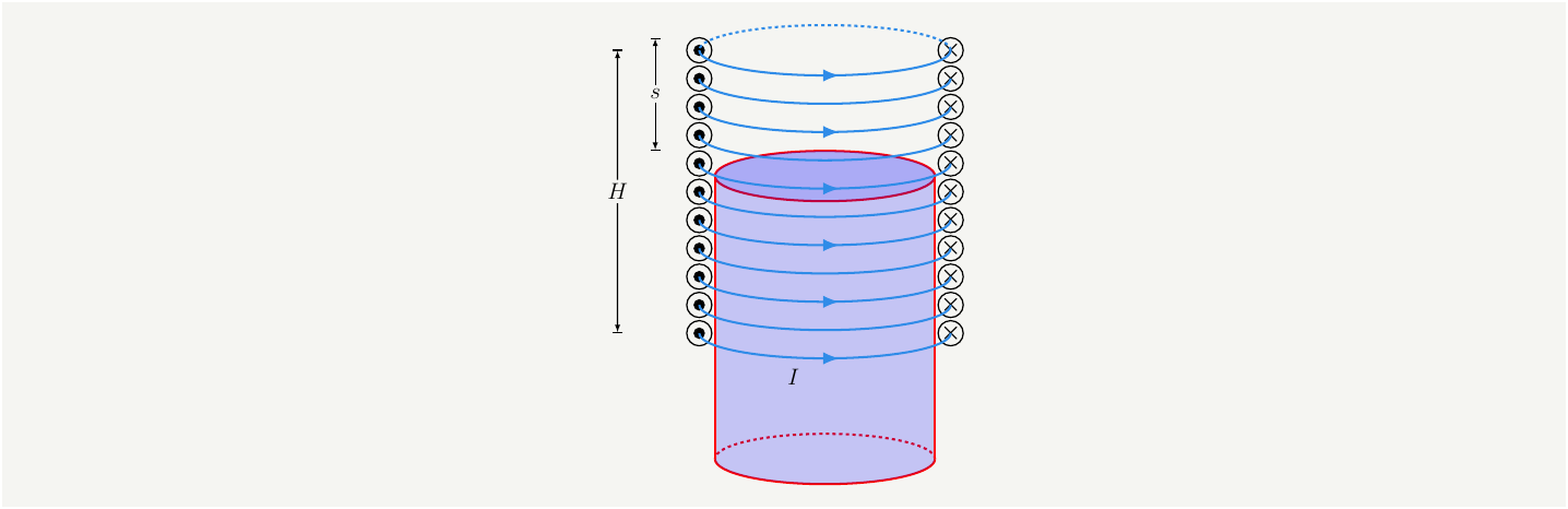
Figure 1: A magnetic material partially inserted inside the coil.
We will need a more sophisticated model to calculate an accurate value for the force, however, we can investigate it qualitatively with this toy model. Note that we labeled the vertical distance that is not filled by the core material as \(s\). The most practical way to compute \(\mathbf{B}\) is to use the concept of magnetomotor force, MMF, which is denoted by \(\mathcal{F}\). In the case of a coil \(\mathcal{F}=N I\), \(N\) is the number of turns and \(I\) is the current. If we express our fields in terms of magnetization field \(\mathbf{H}=\mu\mathbf{B}\), we can write the amperes law as follows: \[\begin{eqnarray} NI=H_c (H-s)+H_0 s =B\frac{H-s}{\mu_c} +B\frac{s }{\mu_0} \tag{1}. \end{eqnarray}\] Solving for \(B\), we get: \[\begin{eqnarray} B=\frac{\mu_r \mu_0 N I}{H}\frac{1}{1+\frac{s}{H}(\mu_r-1) }\tag{2}, \end{eqnarray}\] where \(\mu_r\equiv \mu_c/\mu_0\) is the relative permeability of the core material. The energy density of this setup will be a function of \(s\) and the vertical axis \(z\) since \(\mu\) changes. \[\begin{eqnarray} \mathcal{E}(s,z)=\frac{\mathbf {B}^2(s,z)}{2 \mu(z)} \tag{3}. \end{eqnarray}\] Integrating this over the volume we get \[\begin{eqnarray} E(s)&=&\pi R^2 \int d z \mathcal{E}(s,z) = \pi R^2 \int d z \frac{\mathbf {B}^2}{2 \mu(z) }=\pi R^2 \frac{\mathbf {B}^2}{2} \left[\frac{H-s}{ \mu_c}+\frac{s}{ \mu_0} \right] \nonumber\\ &=& \frac{ \pi R^2 \mu_r \mu_0 N^2 I^2}{2 H}\frac{1}{1+\frac{s}{H}(\mu_r-1) } \tag{4}. \end{eqnarray}\] The force on the material can be calculated simply by taking the derivative of the energy with respect to \(s\):
\[\begin{eqnarray} F(s)=\frac{dE(s)}{ds} &=& -\frac{ \pi R^2 \mu_r^2 \mu_0 N^2 I^2}{2 H^2}\frac{1}{\left(1+\frac{s}{H}(\mu_r-1)\right)^2 } \tag{5}. \end{eqnarray}\] Let’s divide the force by the volume, and re-write it in a slightly different form:
\[\begin{eqnarray} \frac{F(s)}{V}= -\frac{ \mu_r^2 \mu_0 N^2 I^2}{2 H^3}\frac{1}{\left(1+\frac{s}{H}(\mu_r-1)\right)^2 }\propto \frac{(\mu_r N I)^2}{ H^3} \tag{6}. \end{eqnarray}\] What this toy model teaches us is that, the acceleration of the core material, \(\propto \frac{F(s)}{V}\) can be maximized by maximizing this expression \(\frac{(\mu_r N I)^2}{ H^3}\). Note that, not all of the quantities can be varied independently. For example, to support higher currents, we will need thicker wires, which will reduce the number of turns we can fit in a given length \(L\). Furthermore, larger \(N\) will result in larger internal resistance for the coil, limiting the maximum current we can push. We will revisit this when we are modeling a more realistic solenoid.
Including the externals
So far we have ignored the fields outside the coil, but this doesn’t mean they are not important. We can use the MMF technique one more time to understand the effect of the external volume to modify Eq. (1) as follows \[\begin{eqnarray} NI=H_c (H-s)+H_0 s +H^{o}_{eff}L^{o}_{eff} =B\frac{H-s}{\mu_c} +B\frac{s }{\mu_0}+B\frac{L^{o}_{eff} }{\mu_o} \tag{7}, \end{eqnarray}\] where \(H^{o}_{eff}\) represents the average effective field outside the coils, \(L^{o}_{eff}\) is the average effective length the field travels, and finally \(\mu_o\) is the permeability of the material outside. Solving for \(B\), and going through the same steps, we can calculate the force on the core material as:
\[\begin{eqnarray} F(s) &=& -\frac{ \pi R^2 \mu_r^2 \mu_0 N^2 I^2}{2 H^2}\frac{1}{\left(1+\frac{s}{H}(\mu_r-1)+\frac{L^{o}_{eff}}{H} \frac{\mu_c}{\mu_o}\right)^2 } \tag{8}. \end{eqnarray}\] This equation tells us that the force doesn’t simply come from within, it is affected by the properties of the external volume. Qualitatively speaking, the force is determined by the flux we can push through, and that flux is inversely proportional to the reluctance of the whole set up. If we can make the flux travel with ease by reducing the external path to close the magnetic loop, we can increase \(B\). In order to do that, we have this knob: \(\frac{L^{o}_{eff}}{\mu_o}\). We can enclose the solenoid in a magnetic material such that this ratio is minimized.
It is also important to note that the \(s\) dependence of the force will be somewhat accurate only when the core material extends far out from one end, and is inserted well into the coil so that fringe fields are not significant. A more precise calculation requires the computation of fields outside the coil, and that is highly non trivial. However, we will soon argue that a good design should include shields around the coil to localize the external fields. This will also save us from dealing with complicated magnetic fields.
We have extracted a few nuggets of useful information from the toy model:
- The acceleration of the core material can be adjusted by tuning this factor: \((\mu_r N I)^2/L^3\).
- Building a return path for the flux increases the acceleration.
- Eddy losses can be minimized by laminating the conductive material.
All of these observations are implemented in a typical solenoid, as illustrated in Fig. 2
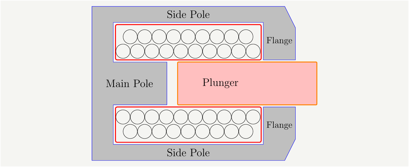
Figure 2: Diagram of a realistic solenoid. Note that this particular set up is designed to pull the plunger inward. It can be modified easily to move the plunger outward. In both cases the modeling will be the same.
Let’s first define a couple o parameters:
- \(H_p\) effective field in the poles,
- \(\mu_p:\) permeability of the poles,
- \(L_p:\) effective length of the poles (main+side+flange),
- \(H_f:\) field in the space between the flange and the plunger,
- \(f_g\): the spacing between the flange and the plunger,
- \(H_{pl}\): The field in the plunger,
- \(\mu_{pl}:\) permeability of the plunger,
- \(L_{pl}\): The maximum length of the plunger that can be placed in the coil.
- \(H_s\): The field in between the main pole and the plunger,
- \(s\): the spacing between the main pole and the plunger.
With these definitions, the MMF equation is now much easier: \[\begin{eqnarray} NI&=&H_p L_p+H_g f_g +H_{pl} L_{pl} + H_s s =B\left(\frac{L_p}{\mu_p} +\frac{f_g }{\mu_0}+\frac{L_{pl}-s }{\mu_{pl}} +\frac{s }{\mu_0}\right) \nonumber\\ &=& B\left(\frac{L_p}{\mu_p} +\frac{f_g }{\mu_0}+\frac{L_{pl}}{\mu_{pl}} +s \left[\frac{\mu_{pl}- \mu_0 }{\mu_0 \mu_{pl}} \right]\right)\equiv B \left(\frac{L_p}{\mu_p} +\frac{f_g }{\mu_0}+\frac{L_{pl}}{\mu_{pl}} \right) \left( 1+\kappa s\right) \tag{9}, \end{eqnarray}\] where we dumped all the mess into the term \(\kappa\): \[\begin{eqnarray} \kappa=\left(\frac{L_p}{\mu_p} +\frac{f_g }{\mu_0}+\frac{L_{pl}}{\mu_{pl}} \right)^{-1} \frac{\mu_{pl}- \mu_0 }{\mu_0 \mu_{pl}} \simeq \left(\frac{L_p}{\mu_p} +\frac{f_g }{\mu_0}+\frac{L_{pl}}{\mu_{pl}} \right)^{-1} \frac{1}{\mu_0} \tag{10}. \end{eqnarray}\]
Since \(\mu_p,\mu_{pl}\gg \mu_0\), we expect \(\kappa\) to be at the order of \(1/f_g\), i.e., the inverse of the spacing between the flange and the plunger. Then magnetic field can be written as: \[\begin{eqnarray} B=\left(\frac{L_p}{\mu_p} +\frac{f_g }{\mu_0}+\frac{L_{pl}}{\mu_{pl}} \right)^{-1} \frac{NI}{\left( 1+\kappa s\right)} \tag{11}, \end{eqnarray}\] The energy of the field reads:
\[\begin{eqnarray} E(s)&=&\int d^3 \mathbf{x} \frac{\mathbf {B}^2(\mathbf{x})}{2 \mu(\mathbf{x})} = \left(\frac{L_p}{\mu_p} +\frac{f_g }{\mu_0}+\frac{L_{pl}}{\mu_{pl}} \right)^{-1} \frac{A N^2I^2}{2 \left( 1+\kappa s\right)} \tag{12}, \end{eqnarray}\] where we picked up similar terms from the integration to reduce quadratic powers to first power. Taking the derivative of the energy with respect to \(s\): \[\begin{eqnarray} F(s)=\frac{dE(s)}{ds} &=& -\left(\frac{L_p}{\mu_p} +\frac{f_g }{\mu_0}+\frac{L_{pl}}{\mu_{pl}} \right)^{-1} \frac{A N^2I^2 \kappa}{2 \left( 1+\kappa s\right)^2} \tag{13}. \end{eqnarray}\] Plugging the expression for \(\kappa\) from Eq. (10), we get
\[\begin{eqnarray} F(s)= -\frac{1}{\mu_0} \left(\frac{L_p}{\mu_p} +\frac{f_g }{\mu_0}+\frac{L_{pl}}{\mu_{pl}} \right)^{-2} \frac{A N^2I^2 }{2 \left( 1+\kappa s\right)^2}= \frac{A B^2(s)}{2 \mu_0} \tag{14}. \end{eqnarray}\]
To get a feel for the magnitude of the force, let’s make some reasonable assumptions and then plug in some numbers:
- Assume high permeability for the the poles and the plunger: Keep \(1/\mu_0\) terms, drop other \(1/\mu\) terms.
- Assume the gap spacing is much larger than the spacing between the flange and the plunger: \(s\gg f_g\).
For this scenario we have \(B=\mu_0 NI/s\) and \(F(s)=\frac{A \mu_0 N^2 I^2}{2 s^2}\).
Let’s take a coil with a certain number of turns and a current such that \(NI=\) 2000, \(A=\) 0.01 \(m^2\), the separation \(s=\) 6 \(mm\). Plugging in these numbers we get: \(F=\) 698 \(N\).
The equation of motion
Consider a case where the solenoid is connected to constant current source. In this case the time dependence of the force in Eq. (13) comes from \(s\), and the equation of motion looks like this: \[\begin{eqnarray} \ddot s= - \frac{C_a}{ \left( 1+\kappa s\right)^2}, \tag{15} \end{eqnarray}\] where \(C_a=\frac{A N^2I^2}{2 m \mu_0} \left(\frac{L_p}{\mu_p} +\frac{f_g }{\mu_0}+\frac{L_{pl}}{\mu_{pl}} \right)^{-2}\). Let’s define \(\dot s =v(s)\), which gives \(\ddot s= \dot v=\frac{dv}{ds}\frac{ds}{dt}=v' \dot s= v' v=\frac{1}{2} \frac{d}{ds}v^2\). Putting this back in
\[\begin{eqnarray} \frac{1}{2} \frac{d}{ds}v^2= - \frac{C_a}{ \left( 1+\kappa s\right)^2} \implies v(s)= -\frac{\sqrt{2 C_a}}{ \sqrt{\kappa( 1+\kappa s)}} \tag{16} \end{eqnarray}\] Integrating once more: \[\begin{eqnarray} t= \frac{1}{\sqrt{2 C_a}}\int_{s}^{s_0} d\tilde s \sqrt{\kappa( 1+\kappa \tilde s) }=\frac{3}{2 \sqrt{2\kappa C_a}}\left[ ( 1+\kappa s_0)^{\frac{3}{2}} -( 1+\kappa s)^{\frac{3}{2}} \right], \tag{17} \end{eqnarray}\] which is the time it takes to move the plunger from its initial position \(s_0\) to an arbitrary position \(s\). Let’s find how long it takes to close the gap completely, i.e., \(s=0\). Let us also assume \(\kappa s_0\gg1\). In this case:
\[\begin{eqnarray} \Delta t=\frac{3 \kappa {s_0}^{\frac{3}{2}} }{2 \sqrt{2 C_a}}, \tag{18} \end{eqnarray}\] In the large permeability limit \(\kappa\simeq \frac{1}{f_g}\) and \(C_a\simeq\frac{A N^2I^2 \mu_0}{2 m f_g^2}\), which give \(\frac{\kappa}{\sqrt{C_a}}=\sqrt{\frac{2m }{A \mu_0}}\frac{1}{NI}\), and we have a simple equation for \(\Delta t\): \[\begin{eqnarray} \Delta t=\frac{3}{2} \sqrt{\frac{m }{A \mu_0}}\frac{1}{NI} {s_0}^{\frac{3}{2}} \tag{19} \end{eqnarray}\]
Consider again a coil with a certain number of turns and a current such that \(NI=\) 2000, \(A=\) 0.01 \(m^2\), \(m\) 50 \(gr\), the separation \(s=\) 6 \(mm\). Plugging in these numbers we get an initial force: \(F=\) 698 \(N\), and the total time: \(\Delta t=\) 0.7 \(ms\). Note that this derivation assumes the current in the wires are kept at a constant value all along. In reality the current will start from \(0\) and will build up slowly depending on the inductance of the system. Therefore the number we got will be underestimating the time. However, the functional form in Eq. (19) is very useful to understand the sensitivity to the parameters we can tune.
Braking mechanism
Unless we are building an electro-mechanical crusher, we will want the plunger to come to a stop at a desired position. In order to do that, all the kinetic energy needs to be dissipated into heat in an harmless manner. In a typical solenoid relay, most of the energy will be lost as the plunger hits to a stopper, and the impact can be dampened by flexible materials and springs. In our case, the speed of the plunger will be \(v\simeq \frac{2 \Delta x}{\Delta t}\simeq \frac{2\times 6 mm}{2 ms}=6m/s\), and at such speeds a stopper might be un desirable since the impact may cause contamination, degradation and failure. Without a stopper, the mechanical energy can still be converted into heat via Eddy currents, as discussed earlier. As the plunger overshoots and extends from the other end of the solenoid, it becomes energetically more favorable for it to be pulled back. Therefore, the plunger will oscillate back and forth, and the magnetic field will change as a response to changing magnetic path resistance. All of these changes will induce Eddy currents in the system, slowly converting the mechanical energy to heat. Eventually the oscillations will die out, and the plunger will settle in its final position.
A self braking mechanism can be implemented as in Fig. 3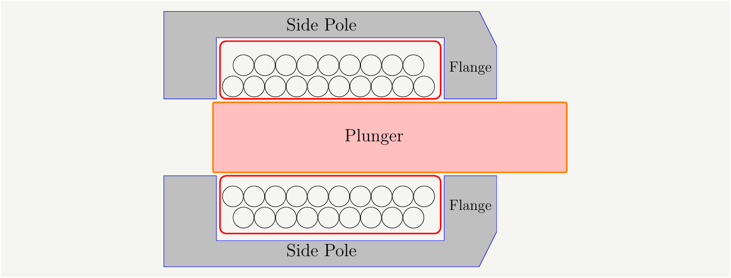
Figure 3: Diagram of a realistic solenoid with self braking.