Consider a random variable \(x(t)\) which evolves with time. The auto correlation function is defined as: \[\begin{eqnarray} C(\tau)=\langle x(t) x(t+\tau)\rangle. \tag{1} \end{eqnarray}\] The Fourier transform of \(C(\tau)\) is defined as \[\begin{eqnarray} \hat C(\omega)=\int_{-\infty}^\infty d \tau e^{-i\omega \tau}C(\tau). \tag{2} \end{eqnarray}\]
Let us define the truncated Fourier transform of \(x(t)\) as \[\begin{eqnarray} \hat x_T(\omega)=\int_{-\frac{T}{2}}^{\frac{T}{2}} dt x(t) e^{-i\omega t}, \tag{3} \end{eqnarray}\] and the truncated spectral power density as \[\begin{eqnarray} S_T(\omega)=\frac{1}{T}\langle |\hat x_T(\omega)|^2\rangle. \tag{4} \end{eqnarray}\] The spectral power density is the limiting case of \(S_T(\omega)\):
\[\begin{eqnarray} S(\omega)=\lim_{T\to \infty}S_T(\omega)=\lim_{T\to \infty}\frac{1}{T}\langle |\hat x_T(\omega)|^2\rangle. \tag{5} \end{eqnarray}\]
The Wiener-Khinchin Theorem states that if the limit in Eq. (5) exists, then the spectral power density is the Fourier transform of the the auto correlation function, i.e., the following equality holds: \[\begin{eqnarray} S(\omega)=\int_{-\infty}^\infty d \tau e^{-i\omega \tau}C(\tau). \tag{6} \end{eqnarray}\]
We start from the average of \(|\hat x_T(\omega)|^2\)
\[\begin{eqnarray} |\hat x_T(\omega)|^2&=&\int_{-\frac{T}{2}}^{\frac{T}{2}} \int_{-\frac{T}{2}}^{\frac{T}{2}}dt' dt \langle x(t') x(t) \rangle e^{-iw(t'-t)}\nonumber\\ &=&\int_{-\frac{T}{2}}^{\frac{T}{2}} \int_{-\frac{T}{2}}^{\frac{T}{2}}dt' dt C(t'-t)e^{-i\omega(t'-t)}. \tag{7} \end{eqnarray}\] Note that \(C(t'-t)e^{-i\omega(t'-t)}\) depends only on the difference of the parameters.
The argument of $the function begs for a change of coordinates:
\[\begin{eqnarray} u=t'-t, \quad \text{and} \quad v=t+t' \tag{8}, \end{eqnarray}\] and the associated inverse transform reads: \[\begin{eqnarray} t'=\frac{u+v}{2}, \quad \text{and} \quad t'=\frac{v-u}{2}. \tag{9} \end{eqnarray}\]
This transformation will rotate and scale the integration domain as shown in Fig. 1.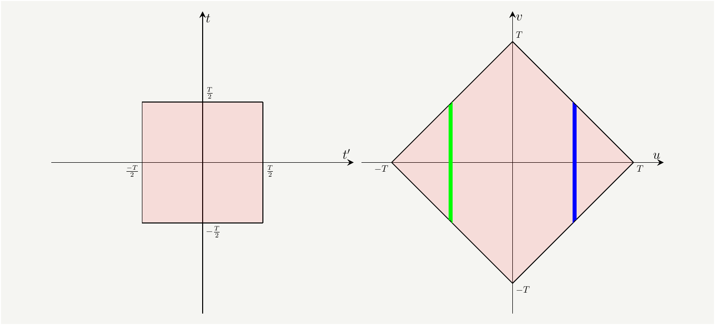
Figure 1: The integration domain in the \(t-t'\) domain (left) and \(u-v\) domain(right). Since there is no \(v\) dependence, \(v\) integration gives the height of the green and blue slices.
The equation of the top boundary on the right can be written as \(v=T-u\), and on the left as $ v= T+u$. We can actually combine them as \(v=T-|u|\). We can do the same analysis for the lower boundaries to see that the height of the slices at a given \(u\) is \(2(T-|u|)\). This will help us easily integrate \(v\) out as follows: \[\begin{eqnarray} I&=&\int_{\frac{-T}{2}}^{\frac{T}{2}}\int_{\frac{-T}{2}}^{\frac{T}{2}} dt' dt f(t'-t) =\iint_{S_{u,v}}\left|\frac{\partial(t,t')}{\partial(u,v)}\right| dv du f(u)\nonumber\\ &=&\int_{-T}^T 2(T-|u|) \times\frac{1}{2} dv du f(u)=\int_{-T}^T du f(u)(T-|u|) \tag{10}, \end{eqnarray}\] where \(\left|\frac{\partial(t,t')}{\partial(u,v)}\right|=\frac{1}{2}\) is the determinant of the Jacobian matrix associated with the transformation in Eq. (9).
Therefore, setting \(u=\tau\), we get \[\begin{eqnarray} |\hat x_T(\omega)|^2&=& \int_{-T}^{T} d\tau e^{-i\omega\tau} C(\tau)(T-|\tau|). \tag{11} \end{eqnarray}\] Taking the average we have the required result: \[\begin{eqnarray} S(\omega)&=&\lim_{T\to \infty}S_T(\omega)=\lim_{T\to \infty}\frac{1}{T}\langle |\hat x_T(\omega)|^2\rangle\nonumber\\ &=& \lim_{T\to \infty}\frac{1}{T}\int_{-T}^{T} d\tau e^{-i\omega\tau} C(\tau)(T-|\tau|)=\int_{-\infty}^{\infty} d\tau e^{-i\omega\tau} C(\tau), \tag{12} \end{eqnarray}\] which completes the proof.