Introduction

The Fabry-Perot interferometer, also known as a Fabry-Perot cavity or etalon, is an optical device that has revolutionized numerous fields in science and technology [1]. Developed by Charles Fabry and Alfred Perot in 1899 [2], it consists of two parallel, highly reflective surfaces separated by a specific distance. Its design allows it to produce sharp interference fringes, making it a powerful tool for high-resolution spectroscopy, laser technology, and precision measurements [3]. The Fabry-Perot interferometer’s ability to selectively transmit or reflect light based on its wavelength has found applications in telecommunications, astronomy, and even in the detection of gravitational waves [4], [5].

The Geometry

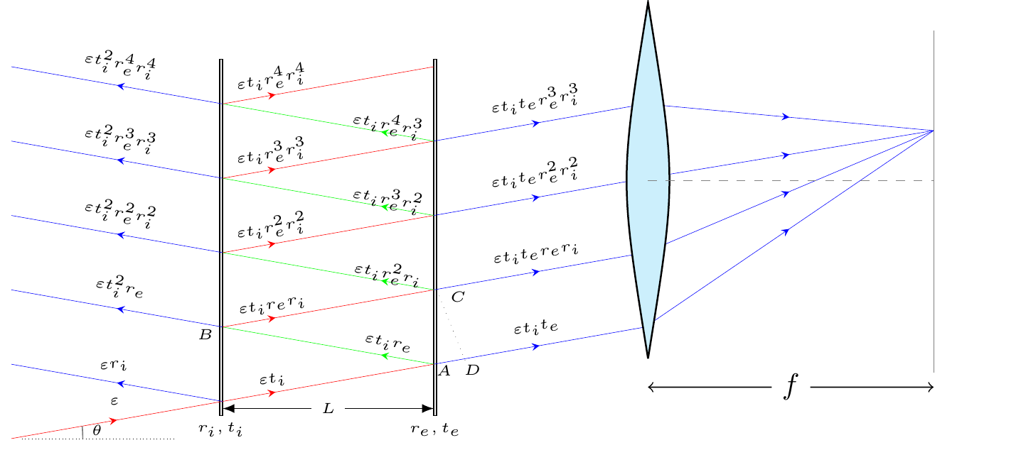
Figure 1: Two semi-reflective mirrors placed in parallel with a distance of \(L\). The light will reflect multiple times between the mirrors.

A plane wave of amplitude \(\varepsilon\) impinges on the setup from the left. Each time the light ray passes through a mirror, it acquires a factor of \(t\), the transmission coefficient, and each time it’s reflected, it acquires a reflection coefficient \(r\). We need to keep track of these factors and sum them up. Another crucial detail is the phase shift as light travels between the mirrors. The distance it covers in a one-way trip is \(L/\cos\theta\). Let’s follow the ray as it splits into two at point \(A\). One portion passes through the mirror and arrives at point \(D\). The remaining part is reflected at point \(A\), then a smaller portion of it is reflected at \(B\) to reach point \(C\). Finally, some of it will transmit through the right mirror.

Note that we must compare the phases at points \(C\) and \(D\), not at \(C\) and \(A\). This is because the wavefront is tilted at an angle \(\theta\). The path difference is:

\[\begin{eqnarray} \Delta= |AB|+|BC|- |AD| \tag{1}. \end{eqnarray}\] It is straightforward to calculate the distances as

\[\begin{eqnarray} |AB|=|BC|=\frac{L}{\cos\theta},\quad |AD|=\sin\theta |AC|= \sin\theta \left( 2\sin\theta |AB|\right)= 2 \sin^2\theta \frac{L}{\cos\theta} \tag{2}. \end{eqnarray}\] Putting these back into Eq. (1), we get \[\begin{eqnarray} \Delta= 2\frac{L}{\cos\theta} \left(1-\sin^2\theta\right)=2L\cos\theta \tag{3}. \end{eqnarray}\] Therefore the phase factor reads: \[\begin{eqnarray} e^{i k 2 L\cos\theta}=e^{i \frac{2\pi L \cos\theta}{\lambda }}\equiv e^{i \theta_T} \tag{4}, \end{eqnarray}\] where \(\lambda\) is the wavelength of the light and we defined \(\theta_T\equiv\frac{2\pi L \cos\theta}{\lambda}\) as the phase shift for one-way travel. Let us now compute the light transmitted all the way to the right side by sum over all the blue arrows pointing right:

\[\begin{eqnarray} \varepsilon_T&=&\varepsilon t_i t_e e^{i \theta_T} +\varepsilon t_i t_e r_e r_i e^{i 3 \theta_T} +\varepsilon t_i t_e r^2_e r^2_i e^{i 5 \theta_T}+\varepsilon t_i t_e r^3_e r^3_i e^{i 7 \theta_T}+\cdots\nonumber\\ &=& \varepsilon t_i t_e e^{i \theta_T} \left\{1+r_e r_i e^{i 2 \theta_T} +\left(r_e r_i e^{i 2 \theta_T}\right)^2+\left(r_e r_i e^{i 2 \theta_T}\right)^3+\cdots\right\} \nonumber\\ &=& \varepsilon t_i t_e e^{i \theta_T} \frac{1}{1-r_e r_i e^{i 2 \theta_T}} \tag{5}. \end{eqnarray}\]

Let’s consider what happens to the phase upon reflection. The phase shifts for two-sided mirrors require careful consideration. For two-sided mirrors, the phase shift occurs for light incident from one side of the mirror. This can be demonstrated using reciprocity arguments, i.e., \(r_L=-r_R\), where \(r_L\) and \(r_R\) are the reflection coefficients for light incident from the left and right sides, respectively.

In our previous calculation, we adopted the conventional approach where the phase shift is defined as \(\pi\) for reflections occurring inside the cavity. However, this phase shift effectively disappears for transmitted rays because there are always an even number of reflections. It’s worth noting that all reflections, except for the very first one, occur inside the cavity. With these considerations in mind, let’s now calculate the reflected beam by summing the blue arrows pointing left: \[\begin{eqnarray} \varepsilon_R&=&\varepsilon r_i -\varepsilon t^2_i r_e e^{i 2 \theta_T} -\varepsilon t^2_i r^2_e r^2_i e^{i 4 \theta_T}-\varepsilon t^2_i r^3_e r^3_i e^{i 6 \theta_T} +\cdots\nonumber\\ &=&\varepsilon r_i -\varepsilon t^2_i r_e e^{i 2 \theta_T}\left\{ 1+ \left( r_e r_i e^{i 2 \theta_T}\right)^2 + \left( r_e r_i e^{i 2 \theta_T}\right)^3 +\cdots \right\} \nonumber\\ &=& \varepsilon r_i -\varepsilon t^2_i r_e e^{i 2 \theta_T}\frac{1}{1-r_e r_i e^{i 2 \theta_T}} \tag{6}, \end{eqnarray}\] where the minus sign is a result of odd number of reflections inside the cavity. Now let’s make use of the conservation of energy:

\[\begin{eqnarray} t^2+r^2+l&=&1 \implies t^2=1-r^2-l \tag{7}, \end{eqnarray}\] where \(l\) is the loss term. Inserting back this back in Eq. (6), we get \[\begin{eqnarray} \varepsilon_R &=& \varepsilon r_i -\varepsilon r_e (1-r^2_i-l_i) e^{i 2 \theta_T}\frac{1}{1-r_e r_i e^{i 2 \theta_T}}= \varepsilon \frac{ r_i -r_e r^2_i e^{i 2 \theta_T}-r_e (1-r^2_i-l_i) e^{i 2 \theta_T}}{1-r_e r_i e^{i 2 \theta_T}}\nonumber\\ &=&\varepsilon \frac{ r_i -r_e (1-l_i) e^{i 2 \theta_T}}{1-r_e r_i e^{i 2 \theta_T}} \tag{8}. \end{eqnarray}\]

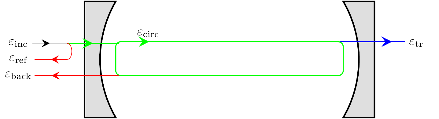
Figure 2: The cavity creates a circulating filed inside. The reflected and transmitted fields can be written in terms of \(E_\text{circ}\) in a recursive way.

\(\varepsilon_\text{circ}\) is the field at the right side of the mirror on the left. It reflects twice and gets a phaseshift to combine back into \(\varepsilon_\text{circ}\). That is: \[\begin{eqnarray} \varepsilon_\text{circ} &=& \varepsilon t_i + r_i r_e e^{i 2 \theta_T} \varepsilon_\text{circ} \implies \varepsilon_\text{circ} =\frac{t_i}{1-r_i r_e e^{i 2 \theta_T}}\varepsilon \tag{9}. \end{eqnarray}\] The transmitted field is easy to write down: \[\begin{eqnarray} \varepsilon_\text{T} &=& t_e e^{i \theta_T} \varepsilon_\text{circ} = \varepsilon e^{i \theta_T}\frac{t_i t_e}{1-r_i r_e e^{i 2 \theta_T}} \tag{10}, \end{eqnarray}\] which is identical to Eq. (5). Similarly for the reflected light, we have \[\begin{eqnarray} \varepsilon_\text{ref} &=& \varepsilon r_i - t_i r_e e^{i 2 \theta_T} \varepsilon_\text{circ} = \varepsilon r_i - t_i r_e e^{i 2 \theta_T}\frac{t_i}{1-r_i r_e e^{i 2 \theta_T}}\varepsilon \tag{11}, \end{eqnarray}\] which is identical to Eq. (6) that led to Eq. (8)

Finesse

Let’s go and play with Eq. (5) a bit.

\[\begin{eqnarray} T\equiv \frac{\varepsilon_T}{\varepsilon}&=& \frac{|t_i t_e|^2}{\left|1-r_e r_i e^{i 2 \theta_T}\right|^2} = \frac{|t_i t_e|^2 }{1-r^2_e r^2_i-2 r_e r_i \cos( 2 \theta_T)} =\frac{|t_i t_e|^2}{\left(1-r_e r_i \right)^2} \frac{1}{1+\frac{4 r_e r_i}{\left(1-r_e r_i \right)^2} \sin^2( \theta_T)} \tag{12}. \end{eqnarray}\] It is periodic and will have its peaks at: \[\begin{eqnarray} \theta_T=\frac{2\pi L \cos\theta}{\lambda }=m\pi \implies \theta_m= \arccos\left(\frac{ m\lambda}{ 2 L}\right) \tag{13}, \end{eqnarray}\]

where \(m\) is an integer. To clean up the notation a bit, let’s define \[\begin{eqnarray} \Phi\equiv \frac{4 r_e r_i}{\left(1-r_e r_i \right)^2} \tag{14}, \end{eqnarray}\] which will transform the transmission coefficient to \[\begin{eqnarray} T=\frac{|t_i t_e|^2}{\left(1-r_e r_i \right)^2} \frac{1}{1+\Phi \sin^2( \theta_T)} \tag{15}. \end{eqnarray}\] It is convenient to define an angle, \(\theta^*_T\) at which \(T\) is equal to the half of its peak value. The peak value is \(T_p=\frac{|t_i t_e|^2}{\left(1-r_e r_i \right)^2}\). We require \[\begin{eqnarray} T({\theta^*_T})=\frac{1}{2} T_p=\frac{|t_i t_e|^2}{\left(1-r_e r_i \right)^2} \frac{1}{1+\Phi \sin^2( \theta^{*}_T)}= =\frac{1}{2} \frac{|t_i t_e|^2}{\left(1-r_e r_i \right)^2} \frac{1}{2} \implies \theta^{*}_T=\arcsin{\frac{1}{\sqrt{\Phi}}} \tag{16}. \end{eqnarray}\] The function is symmetric in \(\theta_T\). The width between these two symmetric points of half peak is \(2\theta^{*}_T=2 \arcsin{\frac{1}{\sqrt{\Phi}}}\). Also remember that the spacing of the peaks is \(\pi\). The ratio of the separation of fringes to the width of half peak points is defined as Finesse \[\begin{eqnarray} \mathcal{F}=\frac{\pi}{2\theta^{*}_T}= \frac{\pi}{2\,\arcsin{\frac{1}{\sqrt{\Phi}}} } \tag{17}. \end{eqnarray}\] \(\Phi\) is typically a large number. Therefore \(\arcsin{\frac{1}{\sqrt{\Phi}}}\simeq \frac{1}{\sqrt{\Phi}}\). The finesse can be simplified as \[\begin{eqnarray} \mathcal{F}=\frac{\pi \sqrt{\Phi}}{2 }=\frac{\pi \sqrt{r_e r_i}}{1-r_e r_i } \tag{18}. \end{eqnarray}\]

We can define three modes of operation when \(\lambda=\frac{2 L}{ m \cos\theta}\)[6]

1. Under coupling: \(\varepsilon_\text{ref}>0\) when \(r_i >r_e (1-l_i)\),

2. Optimal coupling: \(\varepsilon_\text{ref}=0\) when \(r_i =r_e (1-l_i)\),

3. Over coupling: \(\varepsilon_\text{ref}<0\) when \(r_i <r_e (1-l_i)\).

For LIGO, the coefficients are \(t_i^2= 0.03\), and \(r^2_e=0.99997\) [6] which give \(\mathcal{F}=208\) for 4km arms. Light storage time in a cavity is defined as \[\begin{eqnarray} \tau=\mathcal{F} \frac{L}{c} \tag{19}, \end{eqnarray}\] which is about \(870\) ms.

Bulls Eye

This discussion is not relevant for LIGO since \(\theta\simeq 0\) for their detector. For spectroscopic applications, \(\theta\) has some variation, and we want to understand how it affects the interference pattern. Let us turn back to Fig. 1, which has a bunch of outgoing rays. If you look at textbooks or popular youtube channels on the topic, they will tell you that when these rays are projected on a screen with a focusing lens, you will get a bullseye pattern, i.e., concentric cirles of fringes, as shown in Fig. 3.

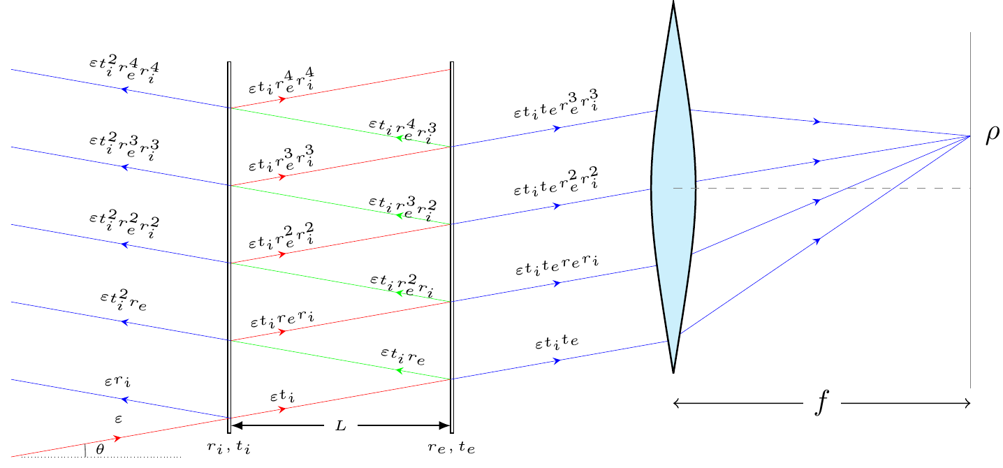
Figure 3: A somewhat-misleading cartoon of the supposed interference pattern when the screen is viewed from front.

This explanation is somewhat misleading. Let’s break it down:

1. If you shine a collimated laser beam of negligible radius into the cavity, you’ll get a series of transmitted beams exiting the cavity that will all be focused to a single point by the lens (ignoring spherical aberration). There’s nothing in Fig. 3 on the source side that would create rings on the screen.

2. To get multiple rings, you need an extended source that provides light at different angles \(\theta\). As you sweep through the source coordinates, the projection on the screen will trace out circles of varying radii \(\rho=f \tan\theta\). The brightness of each ring depends on the interference conditions given by Eq. (5).

To produce the classic bullseye pattern, you need either:

1. An extended source, as shown in Fig. 4 [7], or
2. A divergent beam, which can be created by passing the laser light through a concave lens before it enters the cavity.

These configurations provide the range of incident angles necessary to create the multiple interference rings.

Figure 4: A more realistic illustration of the setup leading to the bullseye pattern. Image taken from [7].

To formulate the interference pattern mathematically, we can write the transfer function, or the Green’s function as physicists will call it, for the system that maps the input rays to points on the screen. It will be something like this:

\[\begin{eqnarray} G(\rho,\phi;\theta',\phi') &=& \delta(\rho-f\tan\theta')\delta(\phi-\phi') T(\theta')=\delta(\rho-f\tan\theta')\delta(\phi-\phi')\frac{|t_i t_e|^2}{\left(1-r_e r_i \right)^2} \frac{1}{1+\Phi \sin^2( \theta'_T)} \tag{20}, \end{eqnarray}\] where, \(\theta'_T=\frac{2\pi L \cos\theta'}{\lambda}\) and we use primed coordinates for the source points. If the source distribution is given by some function, \(S(\theta',\phi')\), the image on the screen will be: \[\begin{eqnarray} I(\rho,\phi)=\int_\text{S} d\theta'd\phi' G(\rho,\phi;\theta',\phi')S(\theta',\phi'), \tag{21} \end{eqnarray}\] where the integral is computed over the source points. Let’s do a test run with a single laser pointer aimed in the direction \((\theta',\phi')=(\theta_L,\phi_L)\); that is: \[\begin{eqnarray} S(\theta',\phi')=S_0 \delta(\theta'-\theta_L)\delta(\phi'-\phi_L), \tag{22} \end{eqnarray}\] where \(S_0\) is the intensity. Plugging this into Eq. (21) we get: \[\begin{eqnarray} I(\rho,\phi)&=&S_0 \int_\text{S} d\theta'd\phi' G(\rho,\phi;\theta',\phi')\delta(\theta'-\theta_L)\delta(\phi'-\phi_L) \nonumber\\ &=& \delta(\rho-f\tan\theta_L)\delta(\phi-\phi_L)\frac{|t_i t_e|^2}{\left(1-r_e r_i \right)^2} \frac{S_0 }{1+\Phi \sin^2( \theta^L_T)}, \tag{23} \end{eqnarray}\] which is a single point at position \(\rho=f \tan\theta_L\) and \(\phi=\phi_L\). The intensity is proportinal to \(1/(1+\Phi \sin^2( \theta^L_T))\), so it may be a dark spot depending on the value of \(\theta^L_T\).

If the input is a cone of light, i.e., it covers \(\phi'\) uniformly; this will remove the \(\delta(\phi-\phi_L)\) from the output, and the result will be \(\propto \delta(\rho-f\tan\theta_L)\), i.e., a ring of \(\rho=f \tan\theta_L\). But, remember, it can be a dark one depending on the value of \(\theta_L\).

Finally, if the source provides a collection of \(\theta'\) rays, now the \(\rho\) will have a range. Let’s say the source is producing somewhat isotropic light of intensity \(S_0\), i.e., uniform for any angle, then we will get the collection of rings: \[\begin{eqnarray} I(\rho,\phi)&=&S_0 \int_\text{S} d\theta'd\phi' G(\rho,\phi;\theta',\phi') =S_0\int_\text{S} d\theta'd\phi' \delta(\rho-f\tan\theta')\delta(\phi-\phi')\frac{|t_i t_e|^2}{\left(1-r_e r_i \right)^2} \frac{1}{1+\Phi \sin^2( \theta'_T)}\nonumber\\ &=&S_0\int_\text{S} d\theta' \delta(\rho-f\tan\theta')\frac{|t_i t_e|^2}{\left(1-r_e r_i \right)^2} \frac{1}{1+\Phi \sin^2( \theta'_T)} \tag{24}. \end{eqnarray}\] Let’s evaluate this integral. First of all we need to deal with the pesky \(\delta(\rho-f\tan\theta')\) term. It will set \(\theta'=\theta_0=\arctan(\rho/f)\), (which also means \(\cos\theta_0=\frac{f}{\sqrt{f^2+\rho^2}}\)), but it will need to figure out the scaling of the integral measure. Let do this dummy shift of variable: \(\theta'=(\theta'-\theta_o) +\theta_0\): \[\begin{eqnarray} \delta(\rho-f\tan\theta')&=&\delta\left(\rho-f \tan\left( (\theta'-\theta_o) +\theta_0\right)\right) =\delta\left(\rho-f\left( \tan \theta_0 +(\theta'-\theta_o) \tan'\theta_0\right)\right) \nonumber\\ &=&\delta\left(f\tan'\theta_0 (\theta'-\theta_o) \right)=\delta\left(\frac{f}{\cos^2\theta_0 }(\theta'-\theta_o) \right)=\frac{\cos^2\theta_0} {f}\delta\left(\theta'-\theta_o \right) \nonumber\\ &=&\frac{f} {f^2+\rho^2}\delta\left(\theta'-\theta_o \right) \tag{25}. \end{eqnarray}\] Putting this back in Eq. (24), we get \[\begin{eqnarray} I(\rho) &=&S_0 \frac{f} {f^2+\rho^2} \frac{|t_i t_e|^2}{\left(1-r_e r_i \right)^2} \left.\frac{1}{1+\Phi \sin^2( \theta'_T)}\right|_{\theta'=\arctan(\rho/f)} \tag{26}. \end{eqnarray}\] Finally, let’s insert the definition of \(\theta'_T\equiv\frac{2\pi L \cos\theta'}{\lambda}\) to write down the final equation: \[\begin{eqnarray} I(\rho) &=& \frac{f S_0} {f^2+\rho^2} \frac{|t_i t_e|^2}{\left(1-r_e r_i \right)^2} \frac{1}{1+\Phi \sin^2\left( \frac{2\pi Lf}{\lambda \sqrt{f^2+\rho^2}}\right)} \tag{27}. \end{eqnarray}\] \(\rho\) is the radial distance from the center, and as it varies we will hit the zeros of \(\sin\) function which will create the bullseye pattern.

Plots

I am working on an interactive plotting tool, which is looks pretty pretty good. I will update the post once it is all done, please check back later.