Johnson–Nyquist noise
Johnson–Nyquist noise (also known as thermal noise, Johnson noise, or Nyquist noise) is the electronic noise generated by the thermal agitation of the charge carriers. This noise exists even when there is no applied voltage. Thermal noise in an ideal resistor is approximately flat. This type of noise was first discovered and measured by John B. Johnson [1], and was later explained by Nyquist[2]. Johnson-Nyquist theorem states that the mean square voltage across a resistor in thermal equilibrium at temperature \(T\) is: \[\begin{eqnarray} \langle V^2\rangle=4R kT \Delta f \tag{1}, \end{eqnarray}\] where \(R\) is the value of the resistance. For complex impedances, the thermal noise is driven by the real part: \[\begin{eqnarray} \langle V^2\rangle=4 \Re \{Z\} kT \Delta f \tag{2}. \end{eqnarray}\]
And finally, if the frequency band is wide, the multiplying factor, \(\Delta f\) needs to be replaced by an integral over the frequency range of interest: \[\begin{eqnarray} \langle V^2\rangle=4 kT \int df \Re \{Z(f)\} \tag{3}. \end{eqnarray}\]
Transmission line derivation
There is a relatively simple derivation of this theorem based on transmission line principles[2]. Consider a resistor \(R\) connected to a matched transmission line, which has the characteristic impedance \(Z_c=R\). The line is terminated with another resistance of value \(R\). The setup is illustrated in Fig. 1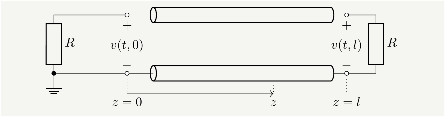
Figure 1: A resistor coupled to a matched transmission line terminated with a resistor of the same value. The whole circuit is kept at a constant temperature \(T\).
The transmission line supports propagating electromagnetic waves, and the energy of these waves are given by the Bose-Einstein statistics: \[\begin{eqnarray} \langle E\rangle=\frac{\hbar\omega}{e^{\frac{\hbar\omega}{kT}}-1} \tag{4}. \end{eqnarray}\] When \(\hbar\omega\ll kT\), we get \(\langle E \rangle=kT\). The rate of energy transmission in a frequency band \(\Delta f\) is \(kT \Delta f\), which is also the power delivered to the load. Therefore the power the load gets is \(kT \Delta f\). In terms of the electrical quantities, the power is given by \(\langle I^2 \rangle R\). Furthermore, we know that \(I=V/(2R)\) due to the resistors in series. Combining all of these pieces, we get the result in Eq.(1).
Microscopic derivation
We are going to follow the method from [3]. Let’s look at a resistor \(R\) with \(N\) electrons per volume; length \(l\); area \(A\), and carrier relaxation time \(\tau_c\). The voltage is given by
\[\begin{eqnarray} V(t)= R I(t)= R A j(t)= R A N e \langle u(t) \rangle, \tag{5} \end{eqnarray}\] where \(I\) is the current, \(j\) is the current density and \(\langle u(t) \rangle\) is the drift velocity. The drift velocity is the average of the individual velocities: \[\begin{eqnarray} \langle u(t) \rangle=\frac{1}{A N l}\sum_i u_i(t), \tag{6} \end{eqnarray}\] where the summation is evaluated over all the electrons with \(u_i\) being individual electron velocity, and the factor in front is the total number of electrons in volume \(A l\). Putting this back in Eq. (5) yields
\[\begin{eqnarray} V(t)= \frac{R e}{l} \sum_i u_i\equiv \sum_i V_i(t), \tag{7} \end{eqnarray}\] where we defined \[\begin{eqnarray} V_i=\frac{R e}{l} u_i \tag{8} \end{eqnarray}\] Since \(u_i\) is a random variable, so is \(V_i(t)\) and we can define an autocorrelation function for them: \[\begin{eqnarray} C_{ij}(\tau)= \langle V_i(t) V_j(t+\tau) \rangle \equiv \delta_{i j}\langle V_i^2 \rangle e^{-|\tau|/\tau_c}. \tag{9} \end{eqnarray}\] The autocorrelation function for the total voltage becomes \[\begin{eqnarray} C_V(\tau)\equiv\langle V(t) V(t+\tau) \rangle &=&\sum_{ij}\langle V_i(t) V_j(t+\tau) \rangle =\sum_{ij}C_{ij}(\tau)= \sum_i \langle V_i^2 \rangle e^{-|\tau|/\tau_c}\nonumber \\ &=& \frac{R^2 e^2}{l^2} \sum_i \langle u_i^2 \rangle e^{-|\tau|/\tau_c} =\frac{R^2 e^2 N A}{l} \langle u^2 \rangle e^{-|\tau|/\tau_c}, \tag{10} \end{eqnarray}\] where we defined the average \(u^2\) over electron velocities as follows: \[\begin{eqnarray} \langle u^2 \rangle= \frac{1}{N A l} \sum_i \langle u_i^2 \rangle \tag{11}. \end{eqnarray}\] Furthermore, we know that in a thermal bath of temperature \(T\), the average kinetic energy of particles are given by the following relation:
\[\begin{eqnarray} \frac{1}{2} m \langle u^2 \rangle= \frac{kT}{2}, \tag{12} \end{eqnarray}\] which implies that \(\langle u^2 \rangle=kT/m\). Plugging this back into Eq. (10), we get the final expression for the correlation:
\[\begin{eqnarray} C_V(\tau)=\frac{R^2 e^2 N A}{l} \frac{kT}{m} e^{-|\tau|/\tau_c}. \tag{13} \end{eqnarray}\]
In order to relate the correlation function \(C_V(\tau)\) to spectral density function, \(S(f)\), we need to do some calculus and prove the Wiener–Khinchin theorem. Since this theorem applies to generic random variables, let us consider a random variable \(x(t)\) which evolves with time. The auto correlation function is defined as: \[\begin{eqnarray} C(\tau)=\langle x(t) x(t+\tau) \rangle. \tag{14} \end{eqnarray}\] The Fourier transform of \(C(\tau)\) is defined as \[\begin{eqnarray} \hat C(\omega)=\int_{-\infty}^\infty d \tau e^{-i\omega \tau}C(\tau). \tag{15} \end{eqnarray}\]
Let us define the truncated Fourier transform of \(x(t)\) as \[\begin{eqnarray} \hat x_T(\omega)=\int_{-\frac{T}{2}}^{\frac{T}{2}} dt x(t) e^{-i\omega t}, \tag{16} \end{eqnarray}\] and the truncated spectral power density as \[\begin{eqnarray} S_T(\omega)=\frac{1}{T}\langle |\hat x_T(\omega)|^2 \rangle. \tag{17} \end{eqnarray}\] The spectral power density is the limiting case of \(S_T(\omega)\):
\[\begin{eqnarray} S(\omega)=\lim_{T\to \infty}S_T(\omega)=\lim_{T\to \infty}\frac{1}{T}\langle |\hat x_T(\omega)|^2\rangle. \tag{18} \end{eqnarray}\]
The Wiener-Khinchin Theorem states that if the limit in Eq. (18) exists, then the spectral power density is the Fourier transform of the the auto correlation function, i.e., the following equality holds: \[\begin{eqnarray} S(\omega)=\int_{-\infty}^\infty d \tau e^{-i\omega \tau}C(\tau). \tag{19} \end{eqnarray}\]
We start from the average of \(|\hat x_T(\omega)|^2\) \[\begin{eqnarray} \langle |\hat x_T(\omega)|^2 \rangle&=&\int_{-\frac{T}{2}}^{\frac{T}{2}} \int_{-\frac{T}{2}}^{\frac{T}{2}}dt' dt \langle x(t') x(t) \rangle e^{-iw(t'-t)} =\int_{-\frac{T}{2}}^{\frac{T}{2}} \int_{-\frac{T}{2}}^{\frac{T}{2}}dt' dt C(t'-t)e^{-i\omega(t'-t)}. \tag{20} \end{eqnarray}\] Note that \(C(t'-t)e^{-i\omega(t'-t)}\) depends only on the difference of the parameters.
The argument of the function begs for a change of coordinates:
\[\begin{eqnarray} u=t'-t, \quad \text{and} \quad v=t+t' \tag{21}, \end{eqnarray}\] and the associated inverse transform reads: \[\begin{eqnarray} t'=\frac{u+v}{2}, \quad \text{and} \quad t'=\frac{v-u}{2}. \tag{22} \end{eqnarray}\]
This transformation will rotate and scale the integration domain as shown in Fig. 2.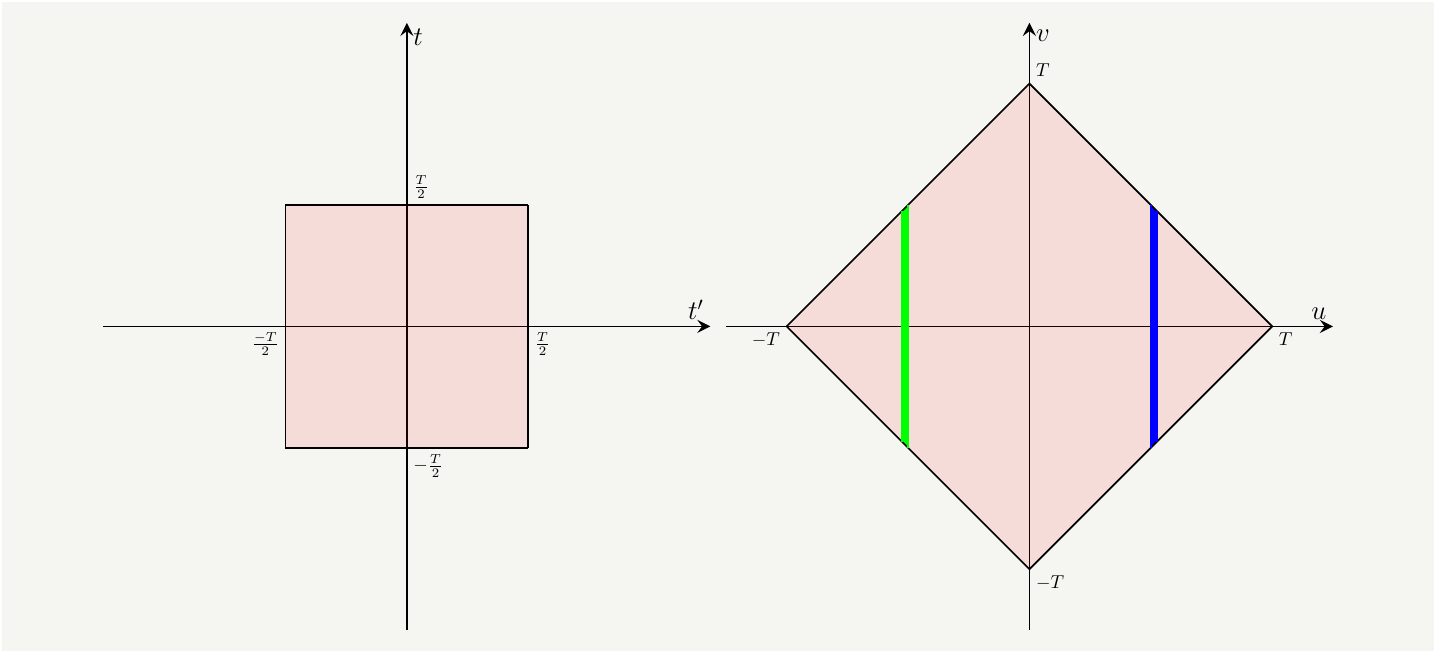
Figure 2: The integration domain in the \(t-t'\) domain (left) and \(u-v\) domain(right). Since there is no \(v\) dependence, \(v\) integration gives the height of the green and blue slices.
The equation of the top boundary on the right can be written as \(v=T-u\), and on the left as $ v= T+u$. We can actually combine them as \(v=T-|u|\). We can do the same analysis for the lower boundaries to see that the height of the slices at a given \(u\) is \(2(T-|u|)\). This will help us easily integrate \(v\) out as follows: \[\begin{eqnarray} I&=&\int_{\frac{-T}{2}}^{\frac{T}{2}}\int_{\frac{-T}{2}}^{\frac{T}{2}} dt' dt f(t'-t) =\iint_{S_{u,v}}\left|\frac{\partial(t,t')}{\partial(u,v)}\right| dv du f(u)\nonumber\\ &=&\int_{-T}^T 2(T-|u|) \times\frac{1}{2} dv du f(u)=\int_{-T}^T du f(u)(T-|u|) \tag{23}, \end{eqnarray}\] where \(\left|\frac{\partial(t,t')}{\partial(u,v)}\right|=\frac{1}{2}\) is the determinant of the Jacobian matrix associated with the transformation in Eq. (22).
Therefore, setting \(u=\tau\), we get \[\begin{eqnarray} |\hat x_T(\omega)|^2&=& \int_{-T}^{T} d\tau e^{-i\omega\tau} C(\tau)(T-|\tau|). \tag{24} \end{eqnarray}\] Taking the average we have the required result: \[\begin{eqnarray} S(\omega)&=&\lim_{T\to \infty}S_T(\omega)=\lim_{T\to \infty}\frac{1}{T}\langle |\hat x_T(\omega)|^2\rangle\nonumber\\ &=& \lim_{T\to \infty}\frac{1}{T}\int_{-T}^{T} d\tau e^{-i\omega\tau} C(\tau)(T-|\tau|)=\int_{-\infty}^{\infty} d\tau e^{-i\omega\tau} C(\tau), \tag{25} \end{eqnarray}\] which completes the proof.
We can now apply it to the correlation function defined in Eq. (13):
\[\begin{eqnarray} S_s(\omega)&=&2 \int_{-\infty}^{\infty} d\tau e^{-i\omega\tau} \frac{ R^2 e^2 N A}{l} \frac{kT}{m} e^{-|\tau|/\tau_c}= \frac{4 R^2 e^2 N A}{l} \frac{kT}{m} \Re \left\{ \int_{0}^{\infty} d\tau e^{-\frac{\tau}{\tau_c}(i\omega \tau_c +1)} \right \}\nonumber\\ &=& \frac{4 R^2 e^2 N A}{l} \frac{kT}{m} \Re \left\{ \frac{\tau_c}{ 1+ i\omega \tau_c } \right \}=\frac{4 R^2 e^2 N A}{l} \frac{kT}{m} \frac{\tau_c}{ 1+ (\omega \tau_c)^2 }, \tag{26} \end{eqnarray}\] where we are dealing with the single-sided spectral density, \(S_s\), which is defined for the positive frequencies and it differs by a factor of \(2\) to yield the same energy when integrated. The order of the relaxation time \(\tau_c\) is typically \(10^{-13}s\), and for low enough frequencies we have \(\omega \tau_c\ll 1\).
In order to eliminate \(\tau_c\) in favor of a more familiar electrical quantity, we need to do some more computation using the drift velocity equation:
\[\begin{eqnarray} m\left(\frac{d}{dt}+\frac{1}{\tau_c} \right)\langle u \rangle =eE \tag{27}, \end{eqnarray}\] where \(E\) is the electric field. The steady state solution of Eq. (27) is simply \(\langle u \rangle= e E\tau_c/m\). The corresponding conductivity can be written as \[\begin{eqnarray} \sigma=\frac{j}{E}=\frac{Ne \langle u \rangle }{E} =N e^2\tau_c/m, \tag{28}. \end{eqnarray}\] which implies \(\tau_c= \frac{m \sigma}{N e^2}\). Plugging this back into Eq. (26) and using \(R=\frac{l}{\sigma A}\), we get the final version of the Johnson-Nyquist formula as in Eq. (1).