RLC filters
The rejection or selection of frequency bands can be easily accomplished by a passive RLC circuit. Figure 1 shows a generic, series RLC circuit.
![A generic RLC circuit driven by an sinusoidal source. The resistance $R$ might be a discrete element or the source resistance. A real inductor comes with series resistance. The boxed element represents a coil. <span class='plus'>... [+]</span> <span class='expanded-caption'> A detailed model of a coil requires more care. We will address that in the following sections.</span>](placeholder.png)
Figure 1: A generic RLC circuit driven by an sinusoidal source. The resistance \(R\) might be a discrete element or the source resistance. A real inductor comes with series resistance. The boxed element represents a coil. … [+]
The steady state analysis of RLC circuits is as easy as manipulating algebraic equations with complex values. For filtering purposes, all we need to do is to analyze the steady state. Transient analysis is much more complicated and will give the full solution. However, all the extra terms in the full solution compared to the steady state one will decay exponentially with time.
Phasor analysis
When a resistor of value \(R\) is under a voltage \(V\), the current through is simply \(V/R\). When a current \(i\) is pushed through an ideal coil of inductance \(L\), the voltage becomes \(V=L\frac{dI}{dt}\). If we take the current as the real part of \(I_0e^{i\omega t}\) we get \(V=i\omega L I\), and the define the impedance as \(Z_L=V/I=i\omega L\). If the serial resistance of \(R_L\) is included to represent a real coil, the impedance becomes \(i\omega L+ R_L\). Finally, the current through a capacitor of capacitance \(C\) is given by \(C\frac{dV}{dt}\), and defining the voltage phasor \(V=V_0e^{i\omega t}\), the current becomes \(i \omega C V\) we get the impedance for the capacitor as \(Z_C=V/I=\frac{1}{i \omega C}\). We will use \(s=i \omega\) to represent complex frequency.
Consider the circuit Fig. 1 for which the total impedance reads:
\[\begin{eqnarray} Z_T&=&R+R_L+Z_C+Z_L=R_T+Z_C+Z_L= R_T+\frac{1}{s C} + s L = \frac{LC s^2 +R_TC s +1}{s C}= L\frac{s^2 +\frac{R_T}{L} s +\frac{1}{LC}}{s }\nonumber\\ &=& L\frac{ s^2 +2\zeta \omega_0 s + \omega^2_0}{s }\tag{1}, \end{eqnarray}\] where we defined \(R_T=R+R_L\), \(\omega_0\equiv\frac{1}{\sqrt{L C}}\) as natural frequency of the oscillation, and \(\zeta\equiv\frac{R_T}{2\sqrt{L/C}}\) as the damping ratio. The current through the circuit is
\[\begin{equation} I=\frac{V_\text{in}}{Z_T}= \frac{V_\text{in}}{L}\frac{s }{ s^2 +2\zeta \omega_0 s + \omega^2_0}\tag{2}. \end{equation}\] We can define the voltage across one of the elements or the sum of voltages across any two elements as the output. For example, let’s take the voltage across the inductor as the output define the transfer function as the ratio of the output voltage and the input voltage to get: \[\begin{equation} H_L(s)=\frac{V_L}{V_\text{in}}=\frac{I (s L+R_L)}{V_\text{in}}= \frac{s^2 +\frac{R_L}{L} s}{ s^2 +2\zeta \omega_0 s + \omega^2_0}\tag{3}. \end{equation}\]
If we define the voltage across the resistor \(R\) as the output [assuming it is a discrete element in the circuit, not the resistance of the voltage source], the transfer function becomes: \[\begin{equation} H_R(s)=\frac{V_R}{V_\text{in}}=\frac{I R}{V_\text{in}}= \frac{R}{L} \frac{s}{ s^2 +2\zeta \omega_0 s + \omega^2_0}\tag{4}. \end{equation}\]
Finally, if we define the voltage across the capacitor as the output, the transfer function becomes: \[\begin{equation} H_C(s)=\frac{V_C}{V_\text{in}}=\frac{I Z_C}{V_\text{in}}= \frac{\omega^2_0}{ s^2 +2\zeta \omega_0 s + \omega^2_0}\tag{5}. \end{equation}\] Note that we can also define the output as the voltage across two elements combined. Although it is rather trivial for passive filters, it is a good exercise to draw the poles and zeros of the transfer function in the complex \(s\) domain. The poles are the same for any transfer function for this circuit, and they are at:
\[\begin{equation} s_\pm= \begin{cases} -\omega_0\left(\zeta \pm \sqrt{\zeta^2-1}\right), & \zeta>1 \\ -\omega_0\left(\zeta \pm i \sqrt{1-\zeta^2}\right), & \zeta<1\\ \pm i \omega_0, & \zeta=1. \end{cases}\tag{6} \end{equation}\] In the interactive tool below, you can adjust the values of the circuit elements, or load one of predefined Filters.
\(f_0(\text{MHz})=\) \(\,\,\zeta=\)
Figure 2: Zero-pole diagram of and the frequency response of the selected RLC filter.
Let’s take a look at the filter at \(45MHZ\), seen in Fig. 3.
Figure 3: A closer look at the filter at 45MHz.
We see that that there is a gain of \(4.5\) or \(13\)dB at around the resonance frequency. But is the maximum gain right at the resonance frequency or is it shifted a bit? You can increase the value of \(R\) to see how the peak moves relative to the resonance frequency. We can also calculate it by taking a closer look at Eq. (3) and calculate is absolute value square as: \[\begin{eqnarray} |H_L(s)|^2&=&\left| \frac{s^2 +\frac{R_L}{L} s}{ s^2 +2\zeta \omega_0 s + \omega^2_0}\right|^2_{s=-i\omega} =\frac{\omega^4 +\frac{R^2_L}{L^2}\omega^2 }{ (\omega^2-\omega^2_0)^2 +4\zeta^2 \omega^2_0 \omega^2 } \tag{7}. \end{eqnarray}\] We take the derivative with respect to \(\omega\), set the result to \(0\) and solve for the critical value of \(\omega\) for small \(R_L\):
\[\begin{eqnarray} \frac{d}{d\omega}|H_L(w)|^2&=& \implies \omega=\omega_0 \frac{1}{\sqrt{1-2 \zeta^2}} -\frac{1}{\omega_0} \frac{R^2_L\zeta^2}{L^2 }+ \text{H.O.T.} \tag{8}, \end{eqnarray}\] which shows that the highes amplification happens at a frequency a bit higher than the natural frequency. This effect might be significant when \(\zeta\) is large.
Transient analysis
This section is included only for completeness and for fun since it is not necessary for filter purposes. There is a one-to-one mapping between the parameters of a mass-spring system and those of an RLC circuit. Figure 4 illustrates this correspondence, and the parameters are described in Table 1.
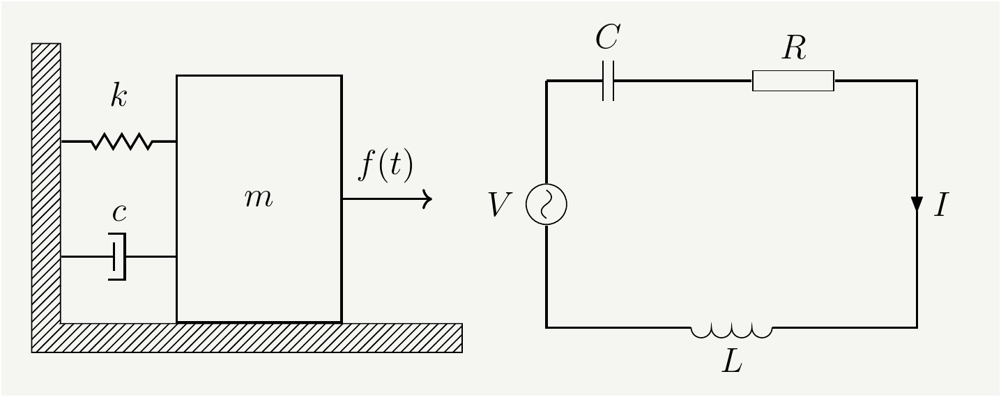
Figure 4: Left:Mass-Spring system with damping driven by an external force, Right: RLC circuit driven by an external voltage source
| Parameter | Description | Parameter | Description |
|---|---|---|---|
| \(k\) | Spring constant | \(C\) | Capacity |
| \(c\) | Damping coefficient | \(R\) | Resistance |
| \(m\) | mass of the object | \(L\) | inductance |
| \(f(t)\) | External force | \(V(t)\) | External Voltage |
Although they are totally different physical systems, the differential equations governing them are very similar, and they can be written as: \[\begin{eqnarray} m \frac{d^2x}{dt^2}+c \frac{dx}{dt}+k x&=&f(t)\quad \text{(Newton's second law)} \tag{9}\\ L \frac{d^2q}{dt^2}+R \frac{dq}{dt}+\frac{ q}{C}&=&V(t)\quad \text{(Kirchhoff's Voltage Law)}\tag{10}. \end{eqnarray}\]
Let’s concentrate on Eq. (10) , and divide the equation by \(L\). The simplified differential equation for forced harmonic oscillator with damping reads: \[\begin{eqnarray} \ddot{q}+ 2\zeta \omega_0 \dot{q}+ \omega_0^2 q&=& \frac{ V(t)}{L} ,\,q(0)=q_0, \,\text{and}\,\dot{q}(0)=\dot{q}_0,\tag{11} \end{eqnarray}\] where \(\dot q\equiv\frac{dq}{dt}\), \(\omega_0\equiv\frac{1}{\sqrt{L C}}\) is the natural frequency of the oscillation, and \(\zeta\equiv\frac{R}{2\sqrt{L/c}}\) is the damping ratio. We also included the initial conditions.
We are dealing with an in-homogeneous linear differential equation with constant coefficients. One of the best tools to solve such equations is the Laplace transformation:
\[\begin{eqnarray} Q(s)=\mathcal{L}\big[q(t)\big]=\int_0^\infty dt \, e^{-s \,t} q(t) \tag{12}. \end{eqnarray}\]
The nice feature of the Laplace transformation is that it converts differential equations to algebraic equations. It follows from the transformation property of the derivatives:
\[\begin{eqnarray} \mathcal{L}\big[\dot{q}(t)\big]&=&\int_0^\infty dt \, e^{-s \,t} \frac{dq}{dt}=\int_0^\infty dt \,\frac{d}{dt}\big(e^{-s \,t} q\big)-\int_0^\infty dt \big(\frac{d}{dt}e^{-s \,t}\big) q\\\nonumber &=& \big(e^{-s \,t} q\big)\bigg\rvert_0^\infty+s\int_0^\infty dt e^{-s \,t} q= s Q(s)- q_0 \tag{13}. \end{eqnarray}\]
Similarly the second order derivative transforms as \[\begin{eqnarray} \mathcal{L}\big[\ddot{q}(t)\big]&=& s \mathcal{L}\big[\dot{q}(t)\big]- \dot{q}_0 =s^2 Q(s) -s q_0 -\dot{q}_0 \tag{14}. \end{eqnarray}\]
Laplace transforming Eq. (11) we get \[\begin{eqnarray} s^2 Q -s q_0 -\dot{q}_0+ 2\zeta \omega_0(s Q- q_0)+\omega_0^2 Q=\frac{ 1}{L} V(s) \tag{15}. \end{eqnarray}\] Solving Eq. (15) for \(Q\), we get
\[\begin{eqnarray} Q&=&\frac{s q_0+ 2\zeta \omega_0q_0+\dot{q}_0}{s^2 +2 \zeta \omega_0 s+\omega_0^2 }+\frac{1}{L}\frac{V(s)}{s^2 +2 \zeta \omega_0 s+\omega_0^2 }\nonumber\\ &=&\frac{(s+ \zeta \omega_0)q_0+ \zeta \omega_0 q_0+\dot{q}_0}{(s + \zeta \omega_0)^2 +\omega_0^2(1 -\zeta^2)}+\frac{1}{L}\frac{V(s)}{(s + \zeta \omega_0)^2 +\omega_0^2(1 -\zeta^2)} \tag{16}. \end{eqnarray}\] The first term in Eq. (16) is related to the initial conditions, and the excitations associated with this term will die out due to damping. The second term relates the response of the system to the external force.
The transfer function of the system is given by \[\begin{eqnarray} H(s)=\frac{Q(s)}{V(s)}\bigg\rvert_{q_0=0=\dot{q}_0}&=&\frac{1}{L}\frac{1}{(s + \zeta \omega_0)^2 +\omega_0^2(1 -\zeta^2)} \tag{17}. \end{eqnarray}\]
Although we will concentrate mostly on the transfer function, it is possible to evaluate the inverse Laplace transform if the functional form of the driving force is known. It is a good exercise to calculate the time domain functions when the system is driven by a sinusoidal force. Let’s assume that \(f(t)\) is of the following form:
\[\begin{eqnarray} v(t)&=&v_0\sin(\omega t). \tag{18} \end{eqnarray}\] Its Laplace transform is given by: \[\begin{eqnarray} V(s)\equiv \mathcal{L}\big[v(t)\big]=\frac{v_0 \omega}{s^2+\omega^2}. \tag{19} \end{eqnarray}\] We will have to do some partial fraction expansion: \[\begin{eqnarray} \frac{1}{\left((s + \zeta \omega_0)^2 +\omega_0^2(1 -\zeta^2)\right)(s^2+\omega^2)}=\frac{A(s+\zeta \omega_0)+B}{(s + \zeta \omega_0)^2 +\omega_0^2(1 -\zeta^2)}+\frac{Cs+D}{s^2+\omega^2}, \tag{20} \end{eqnarray}\] which will be easy to convert back to time domain since they will correspond to sines and cosines with exponential functions in front. We now need to figure out \(A\), \(B\), \(C\) and \(D\). If we were to equate the denominators and sum up the resulting numerators, we will see that, in order to set the coefficient of the \(s^3\) term in the numerator to zero we will need \(A=-C.\) To relate \(C\) and \(D\) we can multiply (20) by \(s-i\omega\) and then set \(s=i\omega.\) This will remove the first term on the right hand side and yield:
\[\begin{eqnarray} i\omega C+D=\frac{1}{(i\omega + \zeta \omega_0)^2 +\omega_0^2(1 -\zeta^2)} \tag{21} \end{eqnarray}\] This is a complex equation, and splitting it into the real and imaginary part, we get: \[\begin{eqnarray} D(\omega_0^2-\omega^2)-2C \omega^2 \omega_0\zeta&=&1\nonumber\\ C\omega(\omega_0^2-\omega^2)+2D \omega \omega_0\zeta&=&0. \tag{22} \end{eqnarray}\] Inverting it, we get: \[\begin{eqnarray} C&=&\frac{-2 \omega_0\zeta}{(\omega_0^2-\omega^2)^2+4\omega^2\omega_0^2\zeta^2}\nonumber\\ D&=&\frac{\omega_0^2-\omega^2}{(\omega_0^2-\omega^2)^2+4\omega^2\omega_0^2\zeta^2} \tag{23} \end{eqnarray}\] Finally, setting \(s=-\zeta \omega_0\), and going trough some algebra we get. \[\begin{eqnarray} B&=&\frac{\omega^2 -\omega_0^2+2\omega_0^2\zeta^2}{(\omega_0^2-\omega^2)^2+4\omega^2\omega_0^2\zeta^2}. \tag{24} \end{eqnarray}\]
We can now inverse transform Eq. (16) using elementary properties of the transformation:
\[\begin{eqnarray} q(t)&=&\mathcal{L}^{-1}\big[Q(s)\big]. \tag{25} \end{eqnarray}\]
Inverse Laplace transformation yields. \[\begin{eqnarray} q(t)&=&\left[q_0 \cos(\omega_0\sqrt{1 -\zeta^2} \,t)+\frac{ \zeta \omega_0 q_0+\dot{q}_0}{\omega_0\sqrt{1 -\zeta^2}}\sin(\omega_0\sqrt{1 -\zeta^2} \,t)\right]e^{-\zeta \omega_0 t}\nonumber\\ &&+\frac{2v_0 \omega}{L}\frac{ \omega_0\zeta}{(\omega_0^2-\omega^2)^2+4\omega^2\omega_0^2\zeta^2}e^{-\zeta \omega_0 t}\cos(\omega_0\sqrt{1 -\zeta^2} \,t)\nonumber\\ &&+\frac{v_0 \omega}{L}\frac{1}{\omega_0\sqrt{1 -\zeta^2}}\frac{\omega^2 -\omega_0^2+2\omega_0^2\zeta^2}{(\omega_0^2-\omega^2)^2+4\omega^2\omega_0^2\zeta^2}e^{-\zeta \omega_0 t}\sin(\omega_0\sqrt{1 -\zeta^2} \,t)\nonumber\\ &&-\frac{2v_0 \omega}{L}\frac{ \omega_0\zeta}{(\omega_0^2-\omega^2)^2+4\omega^2\omega_0^2\zeta^2}\cos(\omega \,t)+\frac{v_0 }{L}\frac{\omega^2 -\omega_0^2}{(\omega_0^2-\omega^2)^2+4\omega^2\omega_0^2\zeta^2}\sin(\omega \,t). \tag{26} \end{eqnarray}\] We can do one last touch and combine the last two terms into as single function with a phase shift.
The full solution with damping, and with \(f(t)=v_0\sin(\omega\, t),\quad\) can be written as: \[\begin{eqnarray} q(t)&=&\left[q_0 \cos(\omega_0\sqrt{1 -\zeta^2} \,t)+\frac{ \zeta \omega_0 q_0+\dot{q}_0}{\omega_0\sqrt{1 -\zeta^2}}\sin(\omega_0\sqrt{1 -\zeta^2} \,t)\right]e^{-\zeta \omega_0 t}\nonumber\\ &+&\frac{v_0 \omega e^{-\zeta \omega_0 t}}{L[(\omega_0^2-\omega^2)^2+4\omega^2\omega_0^2\zeta^2]}\left[2\omega_0\zeta\cos(\omega_0\sqrt{1 -\zeta^2} \,t)+\frac{\omega^2 -\omega_0^2+2\omega_0^2\zeta^2}{\omega_0\sqrt{1 -\zeta^2}}\sin(\omega_0\sqrt{1 -\zeta^2} \,t)\right]\nonumber\\ &+&\frac{ v_0}{L\sqrt{(\omega_0^2-\omega^2)^2+4\omega^2\omega_0^2\zeta^2}}\sin(\omega \,t-\delta) \tag{27} \end{eqnarray}\] where \(\delta\equiv \arctan\left[\frac{2\omega\,\omega_0\zeta}{\omega_0^2-\omega^2}\right]\,\,\), the first line is related to the initial conditions, the second and third lines are the transient response, and finally the last line is the steady state solution.
- At later times, \(t\gg1/(\zeta \omega_0)\), i.e., in the steady state, only the last term survives.
- The \(q(t)\) is sinusoidal, but it will lag by a phase \(\delta\).
- The system will enter in resonance at \(\omega=\omega_0\sqrt{1-2\zeta}\).
- The value of the resonance amplitude is \(v_0/(2\omega_0^2\zeta\sqrt{1-\zeta^2})\).
- At \(\zeta=0\) (no damping), the amplitude diverges. We need to go back and study this case carefully.
Resonances at zero damping: The final solution runs into problems when we consider \(\zeta=0\) and \(\omega=\omega_0\): the coefficient of the steady state solution diverges. This is because of the assumptions we made when we were inverting \(Q(s)\). At \(\zeta=0\) and \(\omega=\omega_0\), two poles will merge and create a second order pole. Let’s take a closer look:
\[\begin{eqnarray} \lim_{\zeta\rightarrow 0,\,\omega\rightarrow\omega_0}\frac{1}{\left((s + \zeta \omega_0)^2 +\omega_0^2(1 -\zeta^2)\right)(s^2+\omega_0^2)}=\frac{1}{(s^2+\omega_0^2)^2}. \tag{28} \end{eqnarray}\] We can figure out how to inverse transform it by exploiting few features of the Laplace transforms as follows:
\[\begin{eqnarray} \mathcal{L}^{-1}\left[\frac{1}{(s^2+\omega_0^2)^2}\right]&=&\mathcal{L}^{-1}\left[-\frac{1}{2s}\frac{d}{ds}\left(\frac{1}{s^2+\omega_0^2}\right)\right]=-\frac{1}{2}\int_0^td\tau \tau \frac{\sin (\omega_0\tau)}{\omega_0}\nonumber\\ &=&-\frac{1}{2 \omega_0}\frac{d}{d\omega_0}\int_0^td\tau \cos (\omega_0\tau)=-\frac{1}{\omega_0}\frac{d}{d\omega_0}\left[\frac{\sin(\omega_0 t)}{\omega_0}\right]=\frac{\sin(\omega_0 t)-\omega_0 t\cos(\omega_0 t)}{2\omega_0^3} \tag{29} \end{eqnarray}\]
The full solution at the resonance frequency (\(\omega=\omega_0\,\) ) with no damping (\(\zeta=0\)) is:
\[\begin{eqnarray} q(t)&=&\left[q_0 \cos(\omega_0\,t)+\frac{\dot{q}_0}{\omega_0}\sin(\omega_0 \,t)\right]+\left[\frac{v_0}{2 m\omega_0^2}\left( \sin(\omega_0 t)-\omega_0 t\cos(\omega_0 t)\right)\right].\tag{30} \end{eqnarray}\] This shows that the amplitude will grow with time. In reality the model will break at some point since the amplitude of oscillations cannot grow indefinitely.
LTspice simulation
One might think that using LTspice for such a simple circuit is an overkill, but this is an opportunity for us to sharpen our tools before we attach the beast! I will pick up a \(9.1\)MHz bandpass filter: \(L=1.8\mu F\), coil resistance \(R_L=2.8\Omega\) (this coil is from CoilCraft, 1008CS-182- more on that later), \(C=174pF\), to be driven by a source with \(23\Omega\) resistance, representing the photodiode. Find the LTspice code here or copy it below.Version 4
SHEET 1 880 680
WIRE 32 48 -112 48
WIRE -112 112 -112 48
WIRE 32 192 32 128
WIRE 32 272 32 256
WIRE 160 272 32 272
WIRE 32 288 32 272
WIRE -112 400 -112 192
WIRE 32 400 32 368
WIRE 32 400 -112 400
WIRE 32 416 32 400
FLAG 32 416 0
FLAG 160 272 Vout9.1
SYMBOL res 16 32 R0
SYMATTR InstName R1
SYMATTR Value 23
SYMBOL voltage -112 96 R0
WINDOW 123 24 152 Left 2
WINDOW 39 24 124 Left 2
SYMATTR Value2 AC 1
SYMATTR SpiceLine Rser=0
SYMATTR InstName V1
SYMATTR Value 0
SYMBOL cap 16 192 R0
SYMATTR InstName C1
SYMATTR Value 174
SYMBOL ind 16 272 R0
SYMATTR InstName L1
SYMATTR Value 1800n
SYMATTR SpiceLine Rser=2.6
TEXT -280 416 Left 2 !.ac dec 10 1 50000000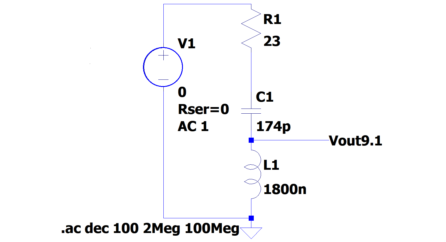
Figure 5: The circuit to simulate in LTspice.
We can run the simulation and look at the frequency response to confirm that it identically matches what we had earlier in the interactive plot. However, this is not the main goal in this subsection.
Launching LTspice
We want to automate the process of running the LTspice via Python. The circuit above is saved as “9_1MHzBP.asc.” One can run LTspice from CMD window by first browsing to the folder that contains the .asc file and run the following command:
"C:\Program Files\LTC\LTspiceXVII\XVIIx64.exe" -Run -b 9_1MHzBP.ascimport sys
import numpy as np
import matplotlib.pyplot as plt
import os
from scipy import interpolate, signal
import filecmp
from shutil import copyfile
import sys
from PyLTSpice.LTSpice_RawRead import RawRead
## Deprecation Warning! This will no longer be supported in future versions.
## Use 'from PyLTSpice import RawWRead' for a direct import of the Raw Reading class
def runLTspice(simname,**kwargs):
theWD = os.getcwd()
target_dir = os.path.dirname(simname)
if( target_dir != ""):
simname = os.path.basename(simname)
os.chdir(target_dir)
verbose = kwargs.get("verbose",False)
interpol = kwargs.get("interpolate",True)
default_ltspice_command = "C:\Program Files\LTC\LTspiceXVII\XVIIx64.exe -Run -b "
if sys.platform == "linux":
default_ltspice_command = 'wine C:\\\\Program\\ Files\\\\LTC\\\\LTspiceXVII\\\\XVIIx64.exe -Run -b '
elif sys.platform == "darwin":
default_ltspice_command = '/Applications/LTspice.app/Contents/MacOS/LTspice -b '
ltspice_command = kwargs.get("ltspice_command",default_ltspice_command)
if sys.platform == "darwin":
simname = simname.replace(".cir","")
else:
simname = simname.replace(".asc","")
if sys.platform == "linux":
os.system(ltspice_command+" {:s}.asc".format(simname))
elif sys.platform == "darwin":
os.system(ltspice_command+" {:s}.cir".format(simname))
else:
import subprocess
subprocess.run([*ltspice_command.split(), "{:s}.asc".format(simname)])
os.chdir(theWD)
runLTspice(f"C:\\Users\\userName\Documents\\github\\aLIGOrfPhotoDetectors\\LSC RFPD Simulation Files\\BluePrints\\2S1N.asc")This will execute simulate the circuit and save a “.raw” file in the same directory, i.e., “9_1MHzBP.raw” in this example.
Parsing LTspice output
We can now parse and analyze this data using PyLTSpice library, which imports the raw file into Python. Find the code here. It works like so:
# A simple example to read simulation results from LT spice
# Get the asc file here:https://github.com/quarktetra/LTspice/blob/main/RLCfilters/9_1MHzBP.asc
# run the following code in CMD (windows OS):
#"C:\Program Files\LTC\LTspiceXVII\XVIIx64.exe" -Run -b 9_1MHzBP.asc
# This will create the   9_1MHzBP.raw file we will use
# 9_1MHzBP.raw is also available here:      https://github.com/quarktetra/LTspice/tree/main/RLCfilters
from PyLTSpice import RawRead    #https://pypi.org/project/PyLTSpice/
import cmath             # dealing with complex numbers
from matplotlib import pyplot as plt
import numpy as np
import os
# make sure the working directory is the one that contains the .asc file.
# if not, you can set below   (requires os)
if False:
    path="path to the directory"
    os.chdir(path)
filepath = '9_1MHzBP.raw'     # will have several columns. We are interested in  frequency and V(vout9.1)
LTR = RawRead(filepath)
## Reading file with encoding utf_16_le
## File contains 8 traces, reading 8
## Binary RAW file with Normal accessprint(LTR.get_trace_names())
#print(LTR.get_raw_property())## ['frequency', 'V(n001)', 'V(n002)', 'V(vout9.1)', 'I(C1)', 'I(L1)', 'I(R1)', 'I(V1)']xa= LTR.get_trace("frequency")
xa=np.asarray(xa).real # converting to np for later analysis
ya= LTR.get_trace("V(vout9.1)")
ya=np.asarray(ya) # this is in complex form, cartesian apparently
ya=np.abs(ya)
plt.plot(xa, ya) #Amplitude vs Freq.
plt.grid(True, which="both", ls="-")
plt.xscale('log')
plt.xlabel("Frequency(Hz)")
plt.ylabel("Gain")
plt.title("Frequency responce of the BandPass filter")
plt.savefig('9_1MHzBP_freq_response.png', dpi=300)
plt.show()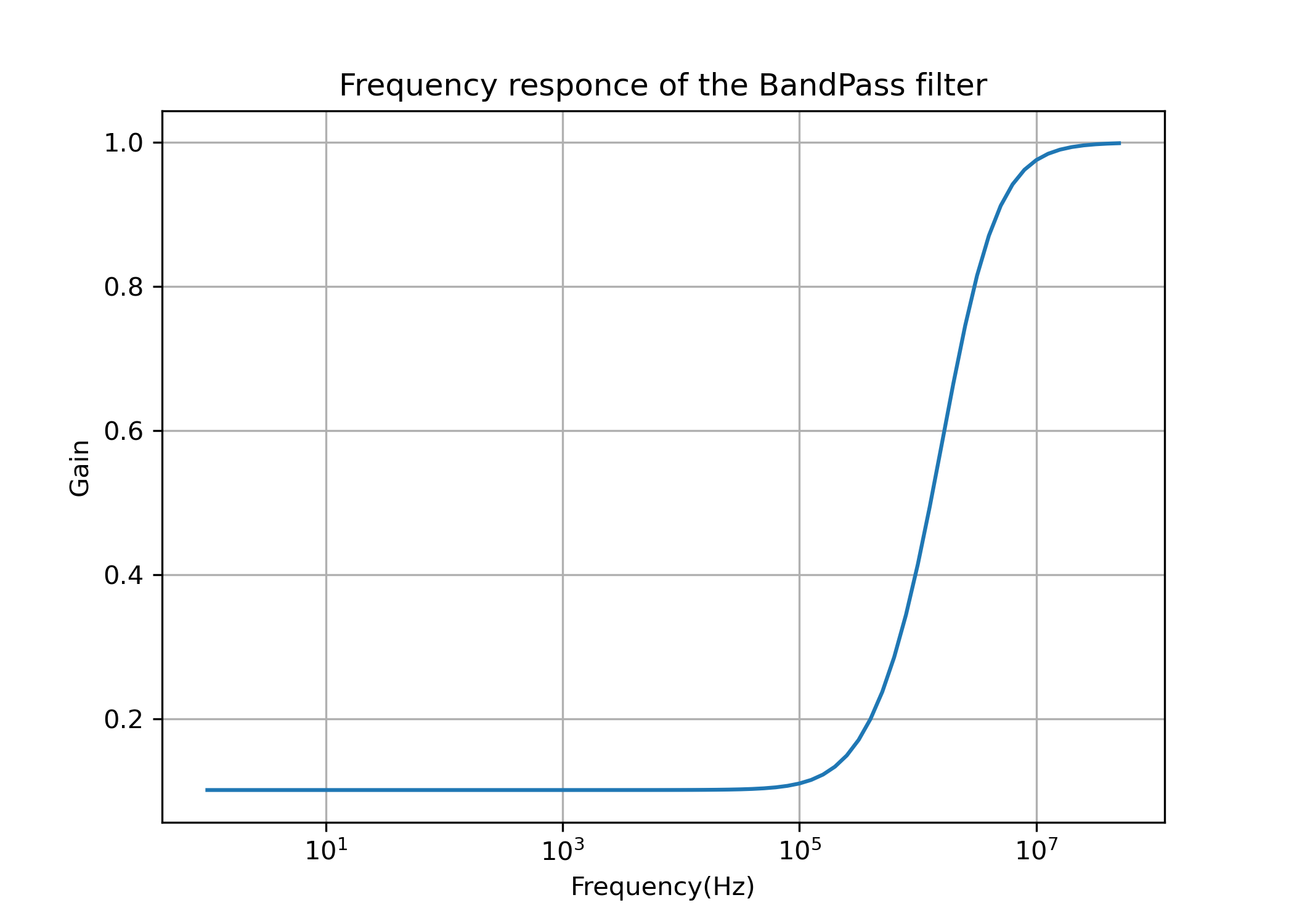
Figure 6: LTspice simulation data.