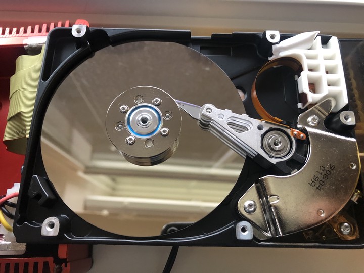
Figure 1: A disk of inner radius \(r_i\) and outer radius \(r_o\) with two sample tracks located at radii \(r_1\) and \(r_2\).
Averaging
Consider two tracks at radii \(r_1\) and \(r_2\) where \(r_{1,2} \in[r_i,r_o]\). The radial distance between them is \(|r_2-r_1|\). If we average over every possible position of \(r_1\) and \(r_2\) we get the average radial distance. Assuming that each \(r\) is equally likely to happen, the density will be \(\frac{1}{r_o-r_i}\), and the average radial distance can be calculated as: \[\begin{eqnarray} \overline{\text{Radial Distance}}&=&\frac{1}{(r_o-r_i)^2}\int_{r_i}^{r_0}\int_{r_i}^{r_0}dr_2dr_1|r_2-r_1|=\frac{2}{(r_o-r_i)^2}\int_{r_i}^{r_0}dr_2\int_{r_i}^{r_2}dr_1(r_2-r_1)\nonumber\\ &=& \frac{2}{(r_o-r_i)^2}\int_{r_i}^{r_0}dr_2\left(r_2(r_2-r_i)-\frac{r_2^2-r_i^2}{2}\right)=2\int_{r_i}^{r_0}dr_2\left(\frac{r_2^2}{2} -r_2r_i+\frac{r_i^2}{2}\right)\nonumber\\ &=& \frac{2}{(r_o-r_i)^2}\left( \frac{r_o^3-r_i^3}{6} -\frac{r_o^2 r_i-r_i^3}{2}+\frac{r_o r_i^2-r_i^3}{2}\right)=\frac{1}{3(r_o-r_i)^2}\left(r_o^3-3 r_0^2 r_i+3 r_or_i^2-r_i^3\right)\nonumber\\ &=&\frac{r_o-r_i}{3}, \tag{1} \end{eqnarray}\] where we used the symmetries of the integral to split the range and convert it to a factor of \(2\).
The integrals were a bit involved since we had nonzero values for both the upper and lower limits. It would be wiser if we define \(r_{1,2}=r_i+\tilde{r}_{1,2}\) and \(\Delta r=r_o-r_i\). This would give a simpler integral to deal with: \[\begin{eqnarray} \overline{\text{Radial Distance}}&=&\frac{1}{(\Delta r)^2}\int^{\Delta r}_{0}\int_{0}^{\Delta r}d\tilde{r}_2d\tilde{r}_1|\tilde{r}_2-\tilde{r}_1|=\frac{2}{(\Delta r)^2}\int_{0}^{\Delta r}d\tilde{r}_2\int_{0}^{\tilde{r}_2}d\tilde{r}_1(\tilde{r}_2-\tilde{r}_1)\nonumber\\ &=&\frac{2}{(\Delta r)^2}\int^{\Delta r}_{0}d\tilde{r}_2 \frac{\tilde{r}_2^2}{2}=\frac{\Delta r}{3}=\frac{r_o-r_i}{3}. \tag{2} \end{eqnarray}\] We are treating the radius as a continuous variable although in an HDD tracks are placed in discrete steps. Would it make any difference if we used discrete math? In that case we just need to switch to indices and summations. Let us define \(r_1= r_i+\Delta \, j\), where \(\Delta\) is the radial separation of two adjacent tracks, and \(j\in[0,N-1]\) is an integer that labels the \(N\) tracks on the disk. The probability of landing on a particular track is \(1/N\). The averaging becomes: \[\begin{eqnarray} \overline{\text{Radial Distance}}&=&\frac{\Delta}{N^2}\sum_{k=0}^{N-1}\sum_{j=0}^{N-1}|k-j|=\frac{2\Delta}{N^2}\sum_{k=0}^{N-1}\sum_{j=0}^{k-1}(k-j)=\frac{2\Delta}{N^2}\sum_{k=0}^{N-1}\left(k^2-\frac{k(k-1)}{2}\right)=\frac{\Delta}{N^2}\sum_{k=0}^{N-1}\left(k^2+k\right)\nonumber\\ &=&\frac{ \Delta}{N^2}\left(\frac{(N-1)N(2N-1)}{6}+\frac{N(N-1)}{2} \right)=\frac{N\Delta}{3}\left(1+ \mathcal{O}(\frac{1}{N})\right)=\frac{r_o-r_i}{3}, \tag{3} \end{eqnarray}\] where \(\mathcal{O}(\frac{1}{N})\) represents the terms of order \(1/N\) or smaller. Since the number of tracks on an HDD disk surface is at the order of \(10^6\), we can safely drop \(1/N\) terms. Furthermore, since \(\Delta\) is the separation of the tracks, \(N\Delta\) was nothing but the radial distance spanned by the tracks, i.e., \(r_o-r_i\). If we look at the ratio of the mean distance to the maximum distance, \(r_o-r_i\), we get: \[\begin{eqnarray} \frac{\overline{\text{Radial Distance}}}{\text{Maximum Distance} }&=& \frac{1}{3}. \tag{4} \end{eqnarray}\] Now that we have shown in multiple ways that average radial distance is \(1/3\) of the maximal distance, we will proceed to show that what we got is not exactly what we were looking for!
Sampling: tracks vs sectors
There was a non-trivial assumption in the previous section: “… each \(r\) is equally likely to happen”. We baked it into our math when we took the density as \(\frac{1}{r_o-r_i}\) in the integrals, and when we took the density as \(1/N\) in the summations. However, a closer inspection shows that this assumption is in conflict with uniformly distributed sectors across the surface. We can explicitly show that if we uniformly sample from tracks and uniformly sample from the locations on the tracks, i.e., the angles, the resulting distribution on the surface will not be uniform. Let’s do a simulation to confirm. We simply sample radius values in the range \([r_i,r_o]\) from a uniform distribution, and the angle values in the range \([0,2\pi]\), and convert them into Cartesian coordinates \(x\) and \(y\) to plot the density of points on the disk.
  library(MASS);library(plotly);  # A code to simulate seek_time. Last update on 5/23/2021, tetraquark.netlify.app/post/seek_time/seek_time
  library(htmlwidgets)
  file_dir<-paste0(getwd(),"/") #"/Users/imac/Documents/GitHub/tetraquark_c"

  set.seed(15)
  samplesize<-100000;
  r_min<-0.7;r_max<-1.7;delta_r<-r_max-r_min  # set radii info
  radius_samples<-r_min+delta_r*runif(samplesize)  # sample uniformly in the selected range
  angle_samples<-2*pi*runif(samplesize)  # select randomly along the circle
  ax<- radius_samples*cos(angle_samples) # compute x-axis value
  ay <- radius_samples*sin(angle_samples) #compute y-axis value

  densityd <- kde2d(ax, ay, n=50)  # this computes the bins and the densities- basically 2d histogram. Requires library MASS
  xb=densityd$x;yb=densityd$y  # pull the x and y bin values

  # the density is 0 for r<r_min, and jumps to its highest value. Contour plot tries to fill in between with a gradient.
  # this is an artifact. Remove that by removing the data around r_min
  for(i in 1:length(xb)){
    for(j in 1:length(yb)){
      if((xb[i]^2+yb[j]^2< r_min^2+0.2) | (xb[i]^2+yb[j]^2>r_max^2-0.1) ){  densityd$z[i,j]<-NA}
    }
  }


  z<-densityd$z
  x<-densityd$x
  y<-densityd$y

  txt <- as.character(outer(X = x, Y = y, function(x, y)
    glue::glue("r:  {round((x^2+y^2)^0.5,2)}")))

  fig<-plot_ly(
    type = "contour",
    x = x,
    y = y,
    z = z,
    text = txt,
    hovertemplate = "Density: %{z:.2f}<br>x: %{x:.2f}<br>y: %{y:.2f}<br>%{text}<extra></extra>",
    colorscale = 'Jet',
    autocontour = F,
    contours = list(
      start = 0.05,
      end = 0.16,
      size = 0.01
    )
  )


  f <- list(  family = "Courier New, monospace",  size = 18,  color = "#7f7f7f")
  x <- list(  title = "x",  titlefont = f)
  y <- list(  title = "y",  titlefont = f)
  fig <- fig %>% layout(xaxis = x, yaxis = y) %>%
    layout(paper_bgcolor='rgba(0,0,0,0)',paper_bgcolor='rgba(0,0,0,0)')%>%
    colorbar(title = "Density") %>%
    config(displayModeBar = F)


    exported<-export(fig, file = "uniformdist.png");
    file_dir<-paste0(file_dir,"content/post/seek_time/")
    saveWidget(fig, paste0(file_dir,"uniformdist.html"), selfcontained = T, libdir = "lib",
               background="rgba(0,0,0,0)")

    knitr::include_graphics('uniformdist.png', error = FALSE)


  save(densityd, file="densitydata.RData") # save this for later
Figure 2: The probability density of randomly selected points on the disk. The steep gradient shows that uniformly sampled radius and uniformly sampled angle do not yield a uniform distribution on the disk.
As shown in Fig. 2, uniformly sampling radius and angle does not yield a uniform distribution on the disk. This intuitively follows from the fact that sampled points are spreading to a wider area at larger radii. In order to restore the uniform distribution on disk surface, we have to abandon the assumption that “… each \(r\) is equally likely to happen”.
The proper density
If we think a bit harder, we can fix this. Consider a small zone from \(r\) to \(r+\delta r\), with \(\delta r \ll r\). The area of this zone is basically the circumference times the width, that is \(2\pi r \,\delta r\). So the area is growing \(\propto r\). Therefore the probability of landing on this band should grow \(\propto r\), i.e., it is not constant. In fact it should be
\[\begin{equation}
f(r)=\frac{2 r}{r_o^2-r_i^2},
\tag{5}
\end{equation}\]
so that it yields \(1\) when integrated from \(r_i\) to \(r_o\). This also makes sense for HDDs. Assuming that the data is uniformly distributed on the disk surface, more data will be on the outer radius of the disk just because there is more area there. Therefore, as the head looks for random sectors, it will find them more on the outer radius, i.e., larger radii tracks will enter into the averaging with larger weights. We have to go back to square one and do the math all over again with the proper probability distribution for tracks. We plug this into the averaging integrals to get:
\[\begin{eqnarray}
\overline{\text{Radial Distance}}&=&\int_{r_i}^{r_0}\int_{r_i}^{r_0}dr_2dr_1f(r_1)f(r_2)|r_2-r_1|=\frac{2}{(r_o^2-r_i^2)^2}\int_{r_i}^{r_o}dr_2\int_{r_i}^{r_2}dr_1r_1r_2(r_2-r_1)\nonumber\\
&=&\frac{4}{15}(r_o-r_i)\frac{r_o^2+3r_ir_o+r_i^2}{(r_o+r_i)^2}=\frac{4}{15}(r_o-r_i)\left(1+\frac{r_ir_o}{(r_o+r_i)^2}\right)\nonumber\\
&=&\frac{4}{15}(r_o-r_i)\left(1+\frac{\kappa}{(1+\kappa)^2}\right).
\tag{6}
\end{eqnarray}\]
The result suggests that the ratio of the mean distance to the maximum distance is
\[\begin{eqnarray}
\frac{\overline{\text{Radial Distance}}}{\text{Maximum Distance} }&=& \frac{4}{15}\left(1+\frac{\kappa}{(1+\kappa)^2}\right) \,\, \text{where}\,\, \kappa\equiv\frac{r_o}{r_i}.
\tag{7}
\end{eqnarray}\]
This is not as elegant as a simple fixed factor of \(1/3\), but, nevertheless it is the correct one as we will support further below.
Figure 3: The ratio of the mean distance to the maximum distance vs \(\kappa=\frac{r_0}{r_i}\). The marked \(\kappa\) value of 2.43 corresponds to typical disk sizes of outer radius \(r_o=1.7\)" and inner radius \(r_k=0.7\)" .
Brute force solution
We can always use Monte Carlo simulations to compute the results. We can select \(x\) and \(y\) in the range \([-r_o,r_o]\) from uniform distributions, and reject the \(x,y\) pairs that fall outside of the disk. That will certainly result in a uniform coverage of the disk as shown in Fig. 4.
  library(MASS);library(plotly);# A code to simulate seek_time. Last update on 5/23/2021, tetraquark.netlify.app/post/seek_time/seek_time
  library(htmlwidgets)

  set.seed(15)
  samplesize<-500000;
  r_min<-0.7;r_max<-1.7;delta_r<-r_max-r_min  # set radii info
  x_samples<- r_max*runif(samplesize,-1,1)
  y_samples<- r_max*runif(samplesize,-1,1)
  r_samples<-(y_samples^2+x_samples^2)^0.5
  keep<-r_samples<r_max & r_samples>r_min # keep only the radii on the disk
  x_samples<-x_samples[keep]
  y_samples<-y_samples[keep]
  r_samples<-r_samples[keep]

  densitydxy <- kde2d(x_samples, y_samples, n=50)  # this computes the bins and the densities- basically 2d histogram. Requires library MASS
  xb=densitydxy$x;yb=densitydxy$y  # pull the x and y bin values

  # the density is 0 for r<r_min, and jumps to its highest value. Contour plot tries to fill in between with a gradient.
  # this is an artifact. Remove that by removing a sliver of data the data around r=r_min and  r=r_max
  for(i in 1:length(xb)){
    for(j in 1:length(yb)){
      if((xb[i]^2+yb[j]^2< r_min^2+0.2) | (xb[i]^2+yb[j]^2>r_max^2-0.4) ){  densitydxy$z[i,j]<-NA}
     }
  }

  z<-densitydxy$z
  x<-densitydxy$x
  y<-densitydxy$y


  txt <- as.character(outer(X = x, Y = y, function(x, y)
    glue::glue("r:  {round((x^2+y^2)^0.5,2)}")))

  fig<-plot_ly(
    type = "contour",
    x = x,
    y = y,
    z = z,
    text = txt,
    hovertemplate = "Density: %{z:.2f}<br>x: %{x:.2f}<br>y: %{y:.2f}<br>%{text}<extra></extra>",
    colorscale = 'Jet',
    autocontour = F,
    contours = list(
      start = 0.0,
      end = 0.16,
      size = 0.02
    )
  )


  f <- list(  family = "Courier New, monospace",  size = 18,  color = "#7f7f7f")
  x <- list(  title = "x",  titlefont = f)
  y <- list(  title = "y",  titlefont = f)
  fig <- fig %>% layout(xaxis = x, yaxis = y) %>%
    layout(paper_bgcolor='rgba(0,0,0,0)',paper_bgcolor='rgba(0,0,0,0)')%>%
    colorbar(title = "Density") %>%
    config(displayModeBar = F)

  fig


  exported<-export(fig, file = "uniformdistxy.png");
  saveWidget(fig, paste0(file_dir,"uniformdistxy.html"), selfcontained = T, libdir = "lib",
             background="rgba(0,0,0,0)")


  # Let us use first half of the points as r1, and the rest as r2
  r1<-r_samples[c(1:(samplesize/2))]
  r2<-r_samples[c((samplesize/2+1):samplesize )]
  dr<-abs(r1-r2) # this is the radial difference, lets take a look at the histogram
  dr<-dr[!is.na(dr)]


  fig<-plot_ly(x = ~dr,nbinsx = 50,
                 type = "histogram",
                 histnorm = "probability")

  x <- list(  title = "Delta r",  titlefont = f)
  y <- list(  title = "Density",  titlefont = f)
  fig <- fig %>% layout(paper_bgcolor='rgba(0,0,0,0)',paper_bgcolor='rgba(0,0,0,0)')%>% layout(xaxis = x, yaxis = y) %>% layout(xaxis = list(range = c(0.01, 1)))


  save(densitydxy, file="densitydataxy.RData") # save this for later
  save(dr, file="dr.RData") # save this for later


  file_dir<-paste0(getwd(),"/")

  file_dir<-paste0(paste(unlist(strsplit(file_dir,"/"))[c(1:8)],collapse="/"),"/")

  file_dir<-gsub("NA/NA/", "", file_dir)

  file_dir<-paste0(file_dir,"content/post/seek_time/")
  saveWidget(fig, paste0(file_dir,"histo.html"), selfcontained = T, libdir = "lib",
             background="rgba(0,0,0,0)")
Figure 4: The probability density of points constructed from \(x\) and \(y\) values selected from uniform distribution. Once the points that fall out of the disk area are rejected, the disk is uniformly covered. We use \(r_o=1.7\)" and inner radius \(r_k=0.7\)" in the simulation.
We can then select a pair of points \(\vec{r}_1\) and \(\vec{r}_2\), and build the histogram of \(|r_2-r_1|\), as shown in Fig. 5.
Figure 5: The distribution of the difference of two randomly chosen radii \(r_2\) and \(r_1\)
Computing the mean value of the distribution and dividing it by the maximum distance, we get 0.3219 to be compared to 0.3218 as predicted in Eq. (7).
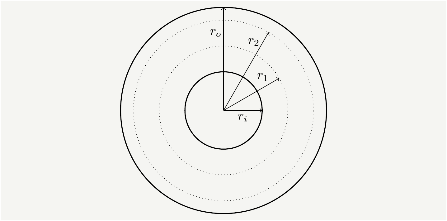
Shut up and calculate!
There is a famous saying among quantum physicist: in most cases quantum behavior becomes so bizarre that there is no intuition that can help you, hence you have to just “shut up and calculate.” I sometimes feel the same way with functions of random variables. In this particular example, we do have an intuitive expectation on the probability distributions and finding out that the distribution we originally used was not uniform on the disk saved the day. However, we would have been in deep trouble if this were a three dimensional problem. It would have been hard to visualize the distributions and/or our intuition might have just failed us. Can’t we just shut up and calculate it formally from the first principles of random variables?
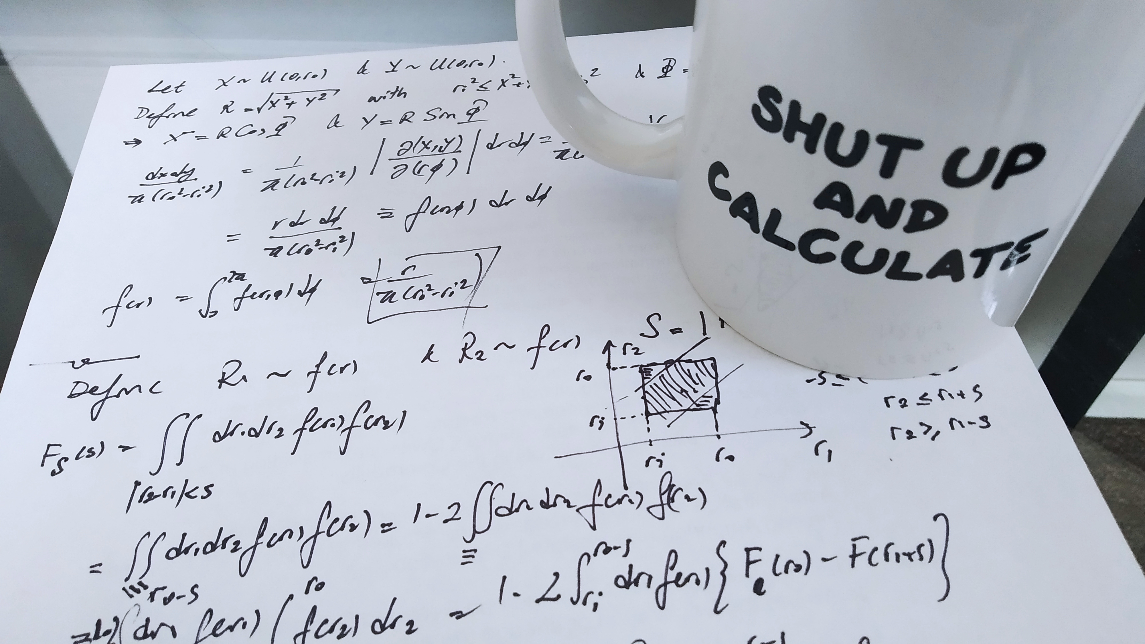
Figure 6: Sometimes it is best to shut up and calculate. Follow the first principles of the theory of random variables and they will lead you to the answer- assuming you don’t screw up the math on the way.
Let us first define the cumulative distribution function \(F(r,\phi)\). We want it to cover the disk uniformly: its increase, let’s call it \(dF\), should be with a uniform rate as we add small portions of area, \(dA=rdrd\phi\). That is: \[\begin{eqnarray} \frac{dF}{dA}=\frac{dF}{rdrd\phi}=c, \tag{8} \end{eqnarray}\] where \(c\) is the normalization constant. It is simply inverse of the disk area: \[\begin{eqnarray} c=\frac{1}{\iint\limits_{\text{disk}}dA}=\frac{1}{\pi(r_o^2-r_i^2)} \tag{9} \end{eqnarray}\] Since there is no \(\phi\) dependence, we can integrate it out and define the radial probability density function: \[\begin{eqnarray} f(r)\equiv\frac{dF}{dr}=\int_0^{2 \pi} d\phi r c= \frac{2 r}{r_o^2-r_i^2}, \tag{10} \end{eqnarray}\] which is identical to Eq. (5).
We can derive the same density function starting from our trusted uniform distribution. Consider two random variables \(X\) and \(Y\) uniformly distributed in the domain defined by \(r^2_i<x^2+y^2<r^2_o\) with the density \(\frac{1}{\pi(r^2_0-r^2_i)}\). We can define two new random variables \(R=(X^2+Y^2)^{1/2}\) and \(\Phi=\text{sign}(Y)\arccos\left(\frac{X}{(X^2+Y^2)^{1/2}}\right)\). The measure of the integral will transform with the Jacobian matrix \[\begin{eqnarray} \frac{dxdy}{\pi(r^2_0-r^2_i)}=\frac{1}{\pi(r^2_0-r^2_i)} \left|\frac{d(x,y)}{d(r,\phi)}\right|drd\phi =\frac{1}{\pi(r^2_0-r^2_i)}\left|\begin{matrix}cos\phi & -r sin\phi \\sin\phi & r \cos\phi\end{matrix}\right|drd\phi =\frac{r}{\pi(r^2_0-r^2_i)}drd\phi. \tag{11} \end{eqnarray}\] Upon integrating out \(\phi\), we pick up a factor of \(2\pi\), and get the same expression for \(f(r)\) as we had in Eqs. (10) and (5).
We have shown in three different ways that the radius, \(R\), will be a random variable with density \(f(r)\). Then we take two such random radii and calculate their radial separation: \(S\equiv|R_1-R_2|\), which is yet another random variable. Figure 5 shows the simulation results for \(S\), and it looks deceptively like a line. However, we do know it can’t be an exact line because then it would have made it a triangle and a triangle has its center of mass at \(1/3\) of the distance from the edge. But we have shown that the real answer deviates from \(1/3\). So we should expect some higher order terms in play.
If we really wanted we could calculate the exact form of the density function of the random variable \(S\). It is best to start from the cumulative distribution: \[\begin{eqnarray} F_S(s)=P(|r_1-r_2|<s)=\iint\limits_{|r_2-r_1|<s}dr_1dr_2 f(r_1)f(r_2). \tag{12} \end{eqnarray}\] We need to figure out the domain for which \(|r_1-r_2|<s\) is satisfied. It is the green shaded area in Fig. 7.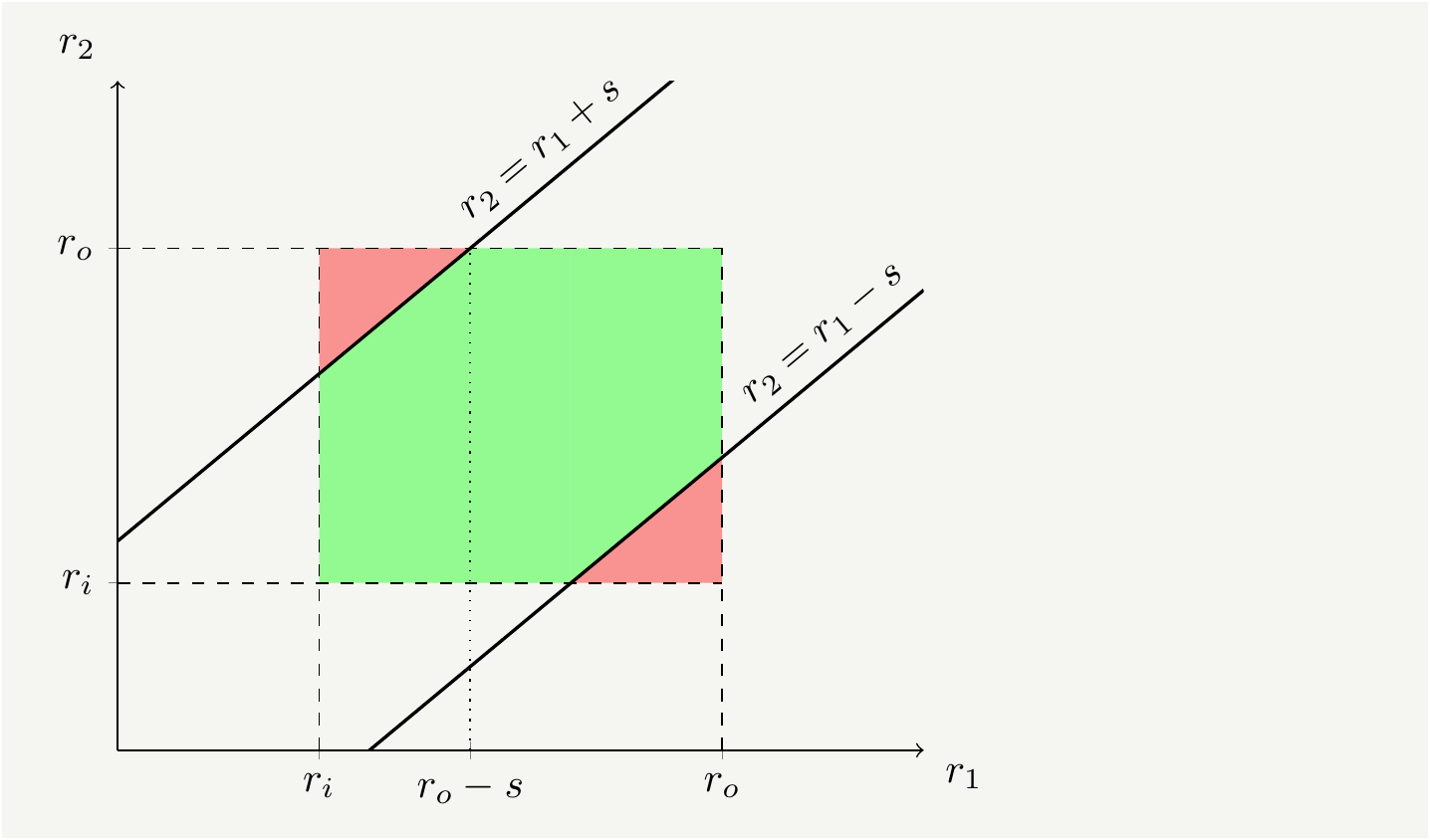
Figure 7: The domain of interest for integration. In the green shaded area \(|r_2-r_1|<s\) is satisfied.
Therefore, the cumulative probability function of the difference can be written as \[\begin{eqnarray} F_S(s)&=&\iint\limits_{|r_2-r_1|<s}dr_1dr_2 f(r_1)f(r_2)= \iint\limits_{\text{green}}dr_1dr_2 f(r_1)f(r_2)=1- \iint\limits_{\text{red}}dr_1dr_2 f(r_1)f(r_2)\nonumber\\ &=&1-2 \int_{r_i}^{r_o-s} dr_1 f(r_1)\int_{r_1+s}^{r_o}f(r_2) dr_2=1-2 \int_{r_i}^{r_o-s} dr_1 f(r_1)\left[ F_R(r_o)-F(r_1+s)\right], \tag{13} \end{eqnarray}\] from which we can get the probability density by differentiating with respect to \(s\): \[\begin{eqnarray} f_S(s)&=&\frac{\partial}{\partial s}F_S(s)=2\int_{r_i}^{r_o-s}dr_1f(r_1)f(r_1+s)=\frac{4}{3\left(r_o^2-r_i^2\right)^2}\left[2(r_o^3-r_i^3)-3(r_o^2+r_i^2)s+s^3 \right]. \tag{14} \end{eqnarray}\] The distribution does differ from a line with a cubic term. \(f_S(s)\) completely defines the statistics of the radial distance of two randomly selected sectors. We can verify that it reproduces the average value by computing \(\frac{1}{r_o-r_i}\int_0^{r_o-r_i}s f(s) ds\), which indeed gives the result in Eq. (7).
Seek time
This post is titled “HDD average seek time,” but so far we have been computing distances. The relation between the distance and the time would have been in a one to one relation if the head moved with constant speed on the radial direction, none of which is exactly true. The head rotates around a pivot point that sits outside the disk, and follows an arc of a circle. Furthermore, it does not move with constant speed as it starts from zero speed, accelerates, slows down and settles at the destination track. Therefore the seek time includes higher order terms. However, we can use the the ratio of average distance to the maximum distance as a proxy to estimate the ratio of average seek time to the time it would take the head to move between the opposite edges of the disk, i.e., the maximum seek time.
Conclusions
HDDs are complicated beasts and in this post we over-simplified few things. An important simplification we made was related to the assumption that the data is uniformly spread on the disk. This is not completely accurate. The capacity density of HDD surfaces has some nontrivial radial dependence [2]. This is an artifact of the skew of the read-write head with respect to the track direction. There are many other effects, which are beyond the scope of this post, that will cause nonuniform distribution of capacity and, in turn the data. In order to address such effects one needs to define \(f(r)\) to incorporate the variations and do the math accordingly.
The bottom line is that it is fair to say that average seek time is about \(1/3\) of the full seek time with certain small and nontrivial deviations.